Voronoi Diagram for Spatial Partitioning — ggplot2

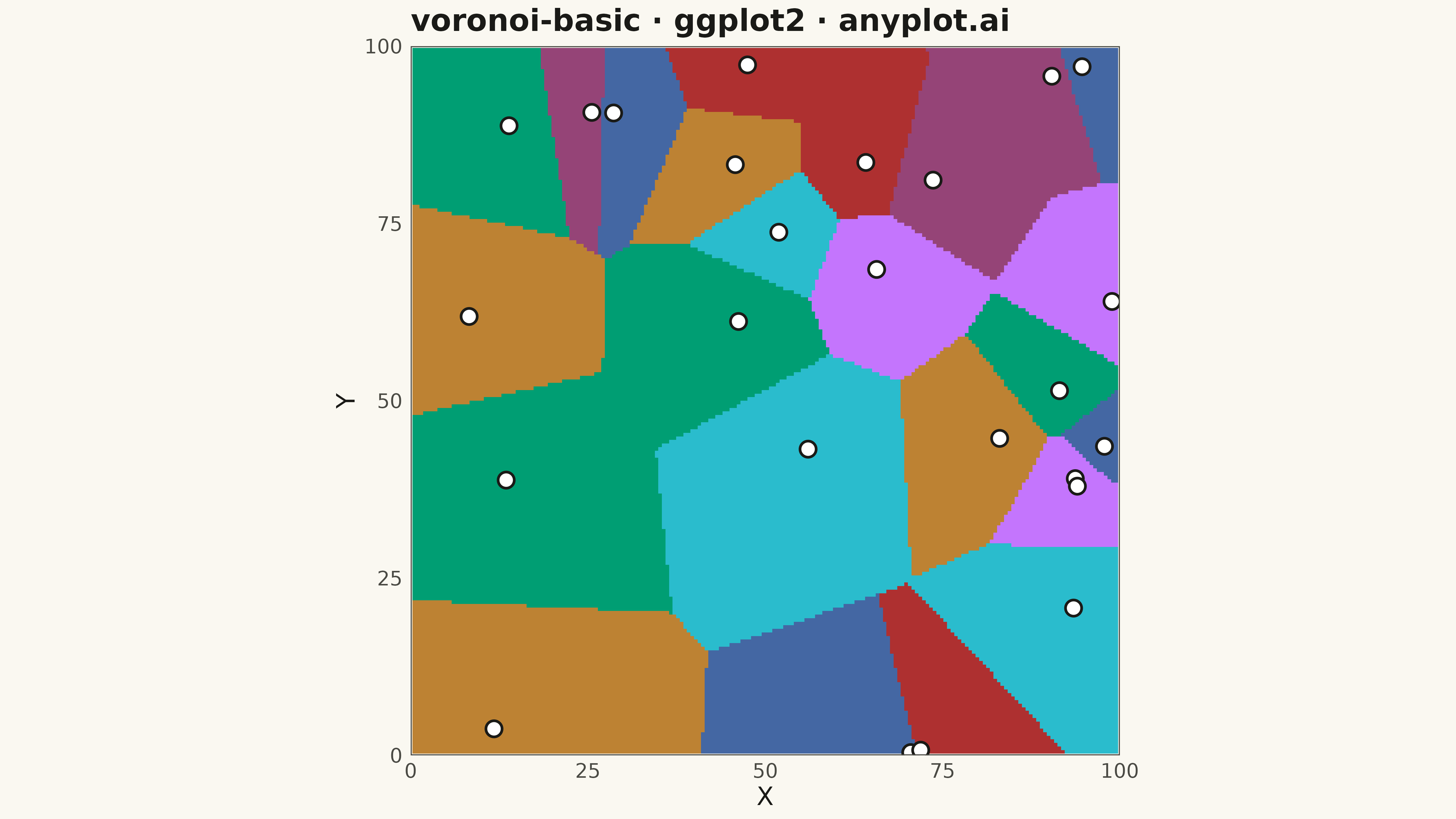
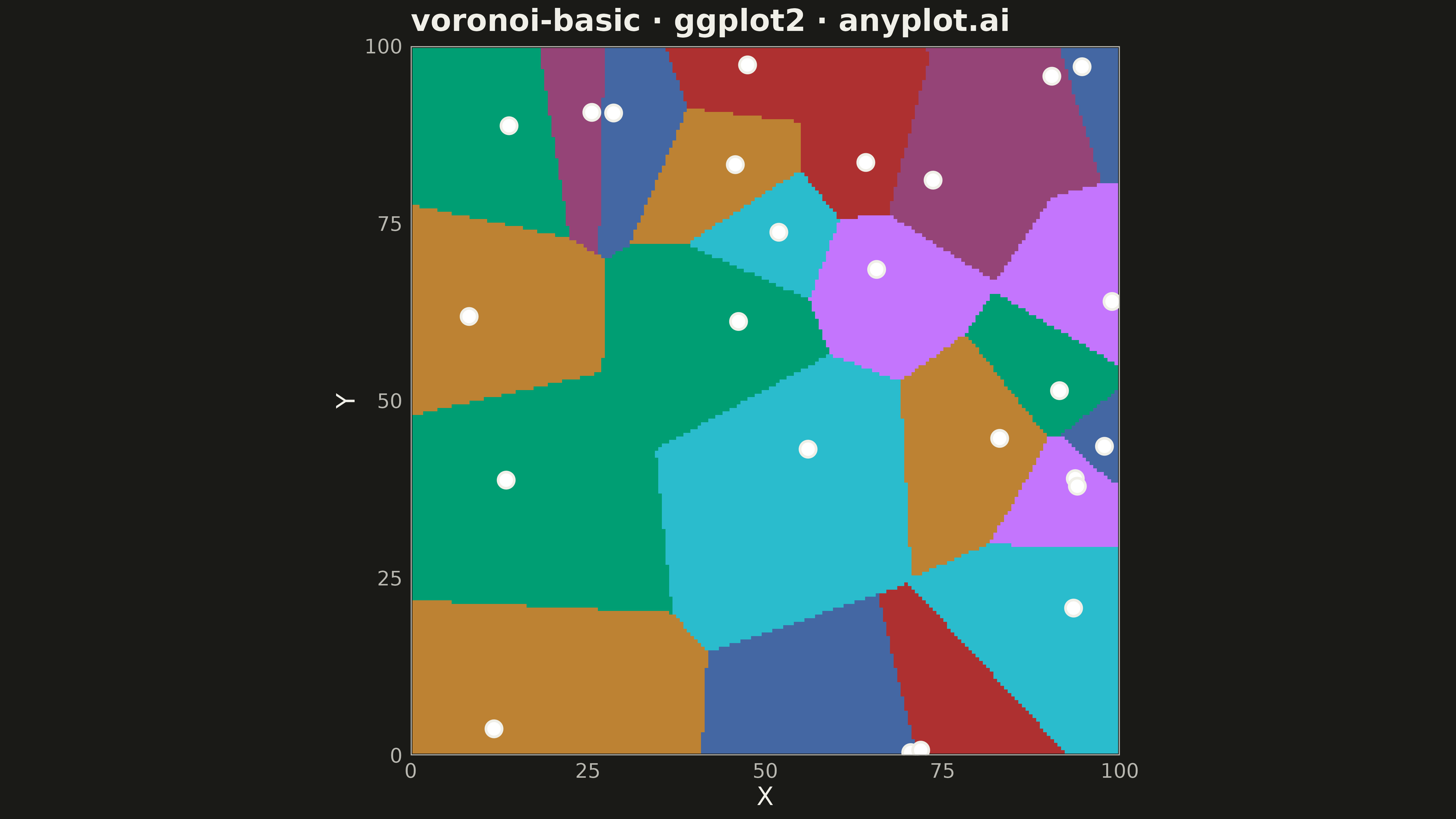
A Voronoi diagram partitions a plane into regions based on the distance to a set of seed points, where each region contains all points closer to its seed than to any other. This visualization is essential for understanding spatial relationships, proximity analysis, and territorial boundaries. It reveals natural clustering patterns and helps identify areas of influence around data points.

Voronoi Diagram for Spatial Partitioning rendered with ggplot2

Renders

R source (ggplot2)

#' anyplot.ai
#' voronoi-basic: Voronoi Diagram for Spatial Partitioning
#' Library: ggplot2 3.5.1 | R 4.4.1
#' Quality: 90/100 | Created: 2026-05-17

library(ggplot2)
library(dplyr)
library(tidyr)
library(ragg)

set.seed(42)

# --- Theme tokens -----------------------------------------------------------
THEME       <- Sys.getenv("ANYPLOT_THEME", "light")
PAGE_BG     <- if (THEME == "light") "#FAF8F1" else "#1A1A17"
ELEVATED_BG <- if (THEME == "light") "#FFFDF6" else "#242420"
INK         <- if (THEME == "light") "#1A1A17" else "#F0EFE8"
INK_SOFT    <- if (THEME == "light") "#4A4A44" else "#B8B7B0"
IMPRINT   <- c("#009E73", "#C475FD", "#4467A3", "#BD8233",
                 "#AE3030", "#2ABCCD", "#954477")

# --- Data: Seed points for Voronoi diagram --------------------------------
n_points <- 25
seed_points <- data.frame(
  id = 1:n_points,
  x = runif(n_points, 0, 100),
  y = runif(n_points, 0, 100)
)

# --- Compute Voronoi cells using distance-based approach ------------------
# Create a fine grid and assign each grid point to its nearest seed
grid_resolution <- 200
grid_df <- expand.grid(
  x = seq(0, 100, length.out = grid_resolution),
  y = seq(0, 100, length.out = grid_resolution)
)

# Calculate distances from each grid point to all seeds
distances <- matrix(NA, nrow = nrow(grid_df), ncol = n_points)
for (i in seq_len(n_points)) {
  distances[, i] <- sqrt(
    (grid_df$x - seed_points$x[i])^2 +
    (grid_df$y - seed_points$y[i])^2
  )
}

# Assign each grid point to the nearest seed
grid_df$region <- apply(distances, 1, which.min)
grid_df$cell_id <- seed_points$id[grid_df$region]

# Join with seed point colors
grid_df <- grid_df %>%
  mutate(
    color_idx = ((cell_id - 1) %% 7) + 1,
    color = IMPRINT[color_idx]
  )

# --- Plot -------------------------------------------------------------------
p <- ggplot(grid_df, aes(x = x, y = y, fill = color)) +
  geom_raster() +
  geom_point(
    data = seed_points,
    aes(x = x, y = y),
    inherit.aes = FALSE,
    color = INK,
    size = 5,
    shape = 21,
    fill = "white",
    stroke = 1.5
  ) +
  scale_fill_identity() +
  scale_x_continuous(limits = c(0, 100), expand = c(0, 0)) +
  scale_y_continuous(limits = c(0, 100), expand = c(0, 0)) +
  coord_fixed() +
  labs(
    title = "voronoi-basic · ggplot2 · anyplot.ai",
    x = "X",
    y = "Y"
  ) +
  theme_minimal(base_size = 14) +
  theme(
    plot.background   = element_rect(fill = PAGE_BG, color = PAGE_BG),
    panel.background  = element_rect(fill = PAGE_BG, color = NA),
    panel.grid.major  = element_blank(),
    panel.grid.minor  = element_blank(),
    panel.border      = element_rect(color = INK_SOFT, fill = NA, linewidth = 0.8),
    axis.title        = element_text(color = INK, size = 20),
    axis.text         = element_text(color = INK_SOFT, size = 16),
    plot.title        = element_text(color = INK, size = 24, face = "bold"),
    legend.position   = "none"
  )

# --- Save -------------------------------------------------------------------
ggsave(
  filename = sprintf("plot-%s.png", THEME),
  plot     = p,
  device   = ragg::agg_png,
  width    = 16,
  height   = 9,
  units    = "in",
  dpi      = 300
)

Part of Voronoi Diagram for Spatial Partitioning on anyplot.ai.

Voronoi Diagram for Spatial Partitioning — ggplot2

Renders

R source (ggplot2)

Other implementations