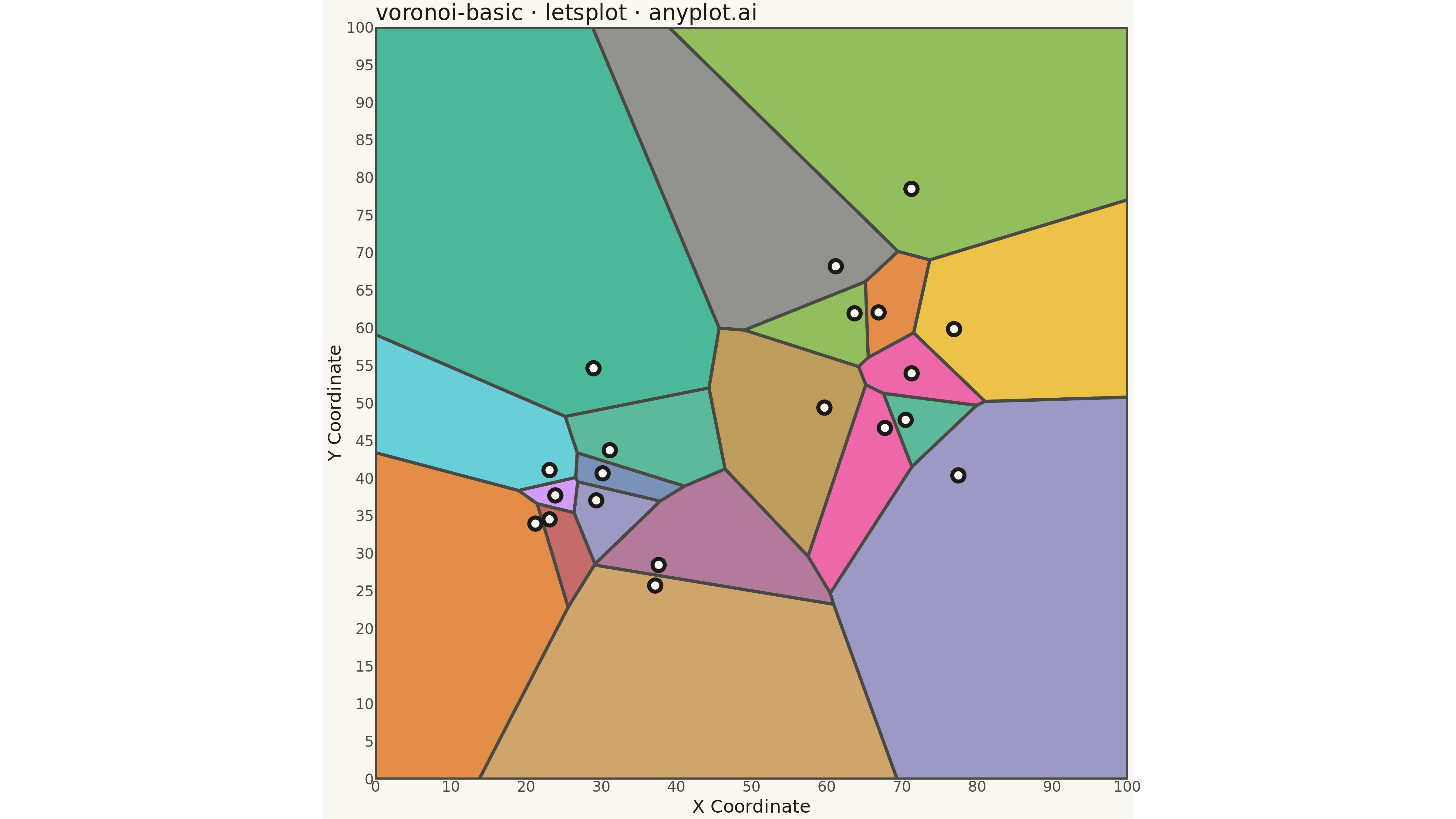
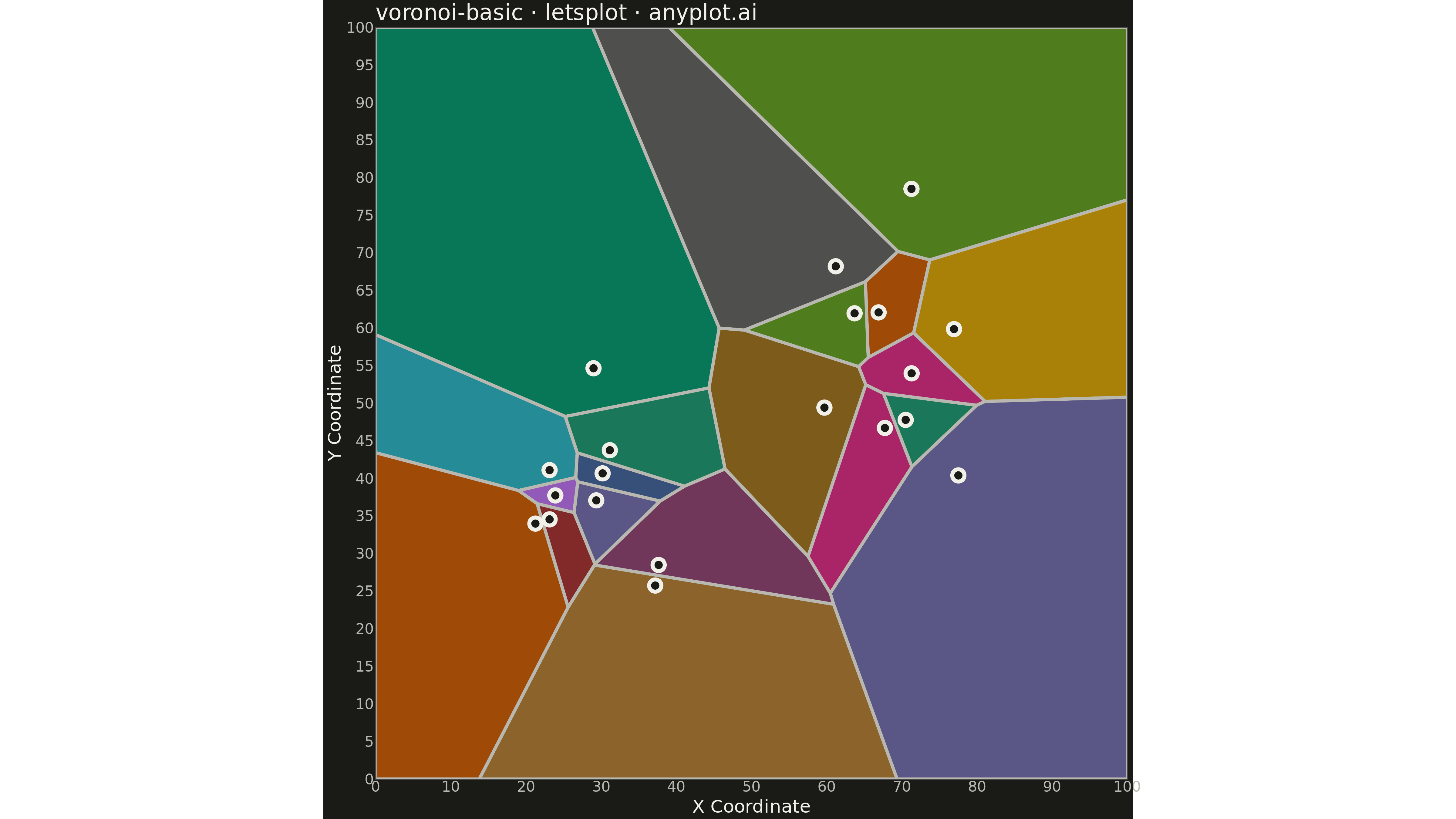
A Voronoi diagram partitions a plane into regions based on the distance to a set of seed points, where each region contains all points closer to its seed than to any other. This visualization is essential for understanding spatial relationships, proximity analysis, and territorial boundaries. It reveals natural clustering patterns and helps identify areas of influence around data points.
""" anyplot.ai
voronoi-basic: Voronoi Diagram for Spatial Partitioning
Library: letsplot 4.9.0 | Python 3.13.13
Quality: 90/100 | Updated: 2026-05-17
"""

import os

import numpy as np
import pandas as pd
from lets_plot import (
    LetsPlot,
    aes,
    coord_fixed,
    element_blank,
    element_line,
    element_rect,
    element_text,
    geom_point,
    geom_polygon,
    ggplot,
    ggsave,
    ggsize,
    labs,
    scale_fill_manual,
    theme,
    theme_minimal,
)
from scipy.spatial import Voronoi


LetsPlot.setup_html()

# Theme tokens
THEME = os.getenv("ANYPLOT_THEME", "light")
PAGE_BG = "#FAF8F1" if THEME == "light" else "#1A1A17"
INK = "#1A1A17" if THEME == "light" else "#F0EFE8"
INK_SOFT = "#4A4A44" if THEME == "light" else "#B8B7B0"

# Data - Generate seed points for spatial partitioning
np.random.seed(42)
n_points = 20

# Generate clustered seed points representing facility locations
x = np.concatenate([np.random.normal(25, 8, n_points // 2), np.random.normal(75, 8, n_points // 2)])
y = np.concatenate([np.random.normal(40, 10, n_points // 2), np.random.normal(60, 10, n_points // 2)])

# Define bounding box for clipping
x_min, x_max = 0, 100
y_min, y_max = 0, 100

# Add boundary points to ensure all regions are clipped
boundary_margin = 200
boundary_points = np.array(
    [
        [x_min - boundary_margin, y_min - boundary_margin],
        [x_min - boundary_margin, y_max + boundary_margin],
        [x_max + boundary_margin, y_min - boundary_margin],
        [x_max + boundary_margin, y_max + boundary_margin],
    ]
)

# Combine seed points with boundary points
all_points = np.column_stack([x, y])
points_with_boundary = np.vstack([all_points, boundary_points])

# Compute Voronoi tessellation
vor = Voronoi(points_with_boundary)

# Build polygon data for each Voronoi region using Sutherland-Hodgman clipping
polygon_data = []
for idx, region_idx in enumerate(vor.point_region[: len(all_points)]):
    region = vor.regions[region_idx]
    if not region or -1 in region:
        continue

    # Get vertices for this region
    vertices = [list(vor.vertices[i]) for i in region]

    # Sutherland-Hodgman polygon clipping to bounding box
    output = vertices
    for edge in ["left", "right", "bottom", "top"]:
        if len(output) == 0:
            break
        input_list = output
        output = []
        for i in range(len(input_list)):
            current = input_list[i]
            previous = input_list[i - 1]

            # Check if point is inside this edge
            if edge == "left":
                curr_inside = current[0] >= x_min
                prev_inside = previous[0] >= x_min
            elif edge == "right":
                curr_inside = current[0] <= x_max
                prev_inside = previous[0] <= x_max
            elif edge == "bottom":
                curr_inside = current[1] >= y_min
                prev_inside = previous[1] >= y_min
            else:  # top
                curr_inside = current[1] <= y_max
                prev_inside = previous[1] <= y_max

            # Compute intersection if crossing edge
            if curr_inside != prev_inside:
                x1, y1 = previous
                x2, y2 = current
                if edge == "left":
                    t = (x_min - x1) / (x2 - x1) if x2 != x1 else 0
                    ix, iy = x_min, y1 + t * (y2 - y1)
                elif edge == "right":
                    t = (x_max - x1) / (x2 - x1) if x2 != x1 else 0
                    ix, iy = x_max, y1 + t * (y2 - y1)
                elif edge == "bottom":
                    t = (y_min - y1) / (y2 - y1) if y2 != y1 else 0
                    ix, iy = x1 + t * (x2 - x1), y_min
                else:  # top
                    t = (y_max - y1) / (y2 - y1) if y2 != y1 else 0
                    ix, iy = x1 + t * (x2 - x1), y_max
                output.append([ix, iy])

            if curr_inside:
                output.append(current)

    # Add clipped polygon vertices to data
    if len(output) >= 3:
        for vx, vy in output:
            polygon_data.append({"x": vx, "y": vy, "region": f"Region {idx + 1}"})

df_polygons = pd.DataFrame(polygon_data)

# Create seed points dataframe
df_seeds = pd.DataFrame({"x": x, "y": y, "label": [f"P{i + 1}" for i in range(len(x))]})

# Color palette for regions - diverse and visually distinct
colors = [
    "#009E73",
    "#C475FD",
    "#4467A3",
    "#BD8233",
    "#AE3030",
    "#2ABCCD",
    "#954477",
    "#1B9E77",
    "#D95F02",
    "#7570B3",
    "#E7298A",
    "#66A61E",
    "#E6AB02",
    "#A6761D",
    "#666666",
    "#1B9E77",
    "#D95F02",
    "#7570B3",
    "#E7298A",
    "#66A61E",
]

# Build plot with Voronoi cells and seed points
plot = (
    ggplot()
    + geom_polygon(data=df_polygons, mapping=aes(x="x", y="y", fill="region"), color=INK_SOFT, size=1.5, alpha=0.7)
    + geom_point(data=df_seeds, mapping=aes(x="x", y="y"), color=INK, size=8)
    + geom_point(data=df_seeds, mapping=aes(x="x", y="y"), color=PAGE_BG, size=4)
    + scale_fill_manual(values=colors)
    + coord_fixed(xlim=[x_min, x_max], ylim=[y_min, y_max])
    + labs(x="X Coordinate", y="Y Coordinate", title="voronoi-basic · letsplot · anyplot.ai")
    + theme_minimal()
    + theme(
        plot_background=element_rect(fill=PAGE_BG, color=PAGE_BG),
        panel_background=element_rect(fill=PAGE_BG),
        panel_grid_major=element_blank(),
        panel_grid_minor=element_blank(),
        plot_title=element_text(size=24, color=INK),
        axis_title=element_text(size=20, color=INK),
        axis_text=element_text(size=16, color=INK_SOFT),
        axis_line=element_line(color=INK_SOFT),
        legend_position="none",
    )
    + ggsize(1600, 900)
)

# Save outputs with theme suffix
ggsave(plot, f"plot-{THEME}.png", path=".", scale=3)
ggsave(plot, f"plot-{THEME}.html", path=".")
Runnable source as JSON, for any HTTP client: https://api.anyplot.ai/specs/voronoi-basic/letsplot/code. Any spec id and library id listed in llms-full.txt fit the same URL shape; every URL below is complete and callable.
{
  "spec_id": "voronoi-basic",
  "language": "python",
  "library": "letsplot",
  "page": "https://anyplot.ai/voronoi-basic/python/letsplot",
  "hub": "https://anyplot.ai/voronoi-basic",
  "code_json": "https://api.anyplot.ai/specs/voronoi-basic/letsplot/code",
  "spec_json": "https://api.anyplot.ai/specs/voronoi-basic",
  "render_light_png": "https://storage.googleapis.com/anyplot-images/plots/voronoi-basic/python/letsplot/plot-light.png",
  "render_dark_png": "https://storage.googleapis.com/anyplot-images/plots/voronoi-basic/python/letsplot/plot-dark.png",
  "interactive_light_html": "https://storage.googleapis.com/anyplot-images/plots/voronoi-basic/python/letsplot/plot-light.html",
  "interactive_dark_html": "https://storage.googleapis.com/anyplot-images/plots/voronoi-basic/python/letsplot/plot-dark.html",
  "quality_score": 90.0,
  "license": "MIT",
  "guide": "https://anyplot.ai/llms.txt"
}
Part of Voronoi Diagram for Spatial Partitioning on anyplot.ai.