The same plot in 14 other libraries — JavaScript: Chart.js, Apache ECharts, Highcharts, MUI X Charts; Python: Altair, Bokeh, lets-plot, Matplotlib, Plotly, plotnine, Pygal, Seaborn; R: ggplot2; Julia: Makie.jl. Compare all 15 side by side: Voronoi Diagram for Spatial Partitioning in Python, R, Julia and JavaScript.
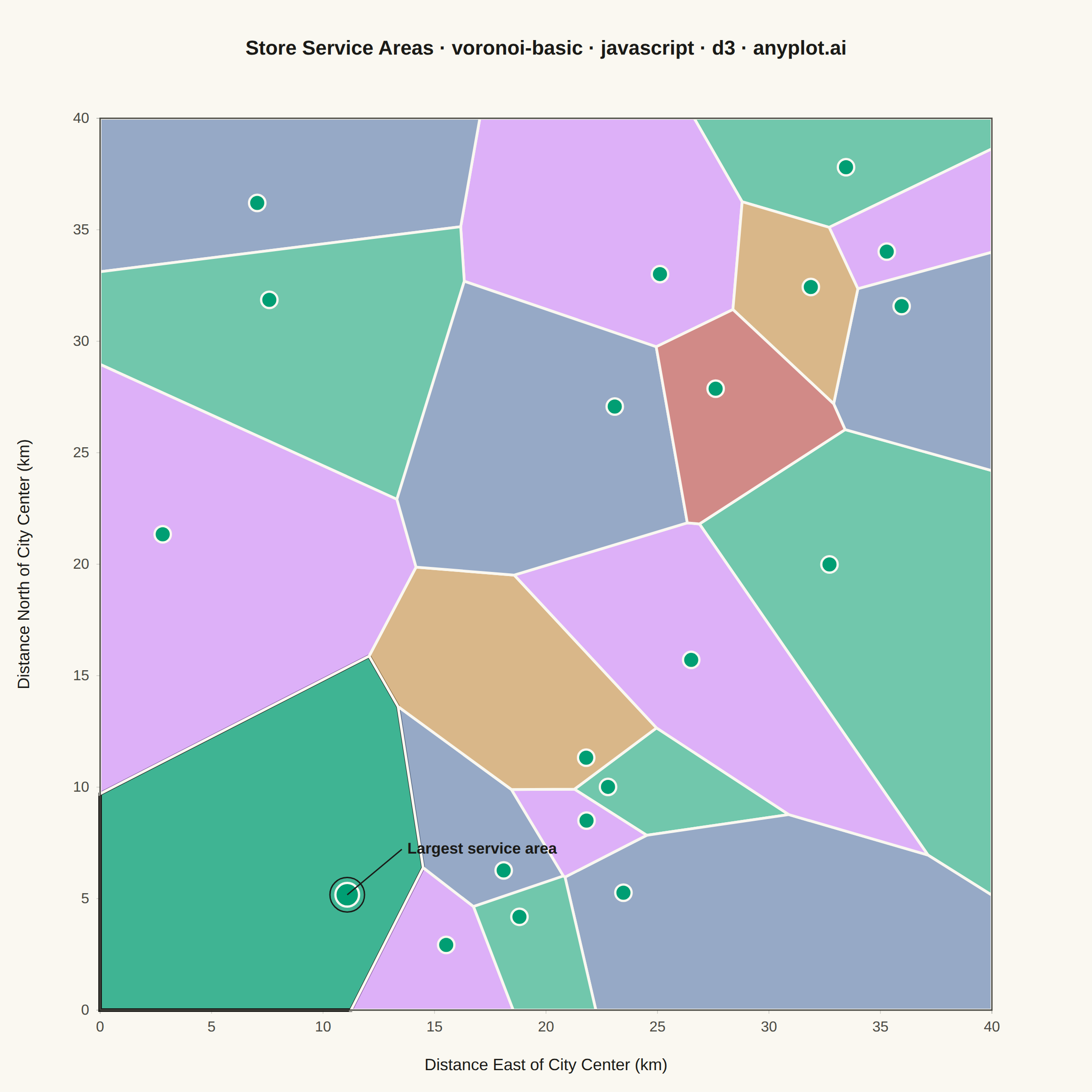
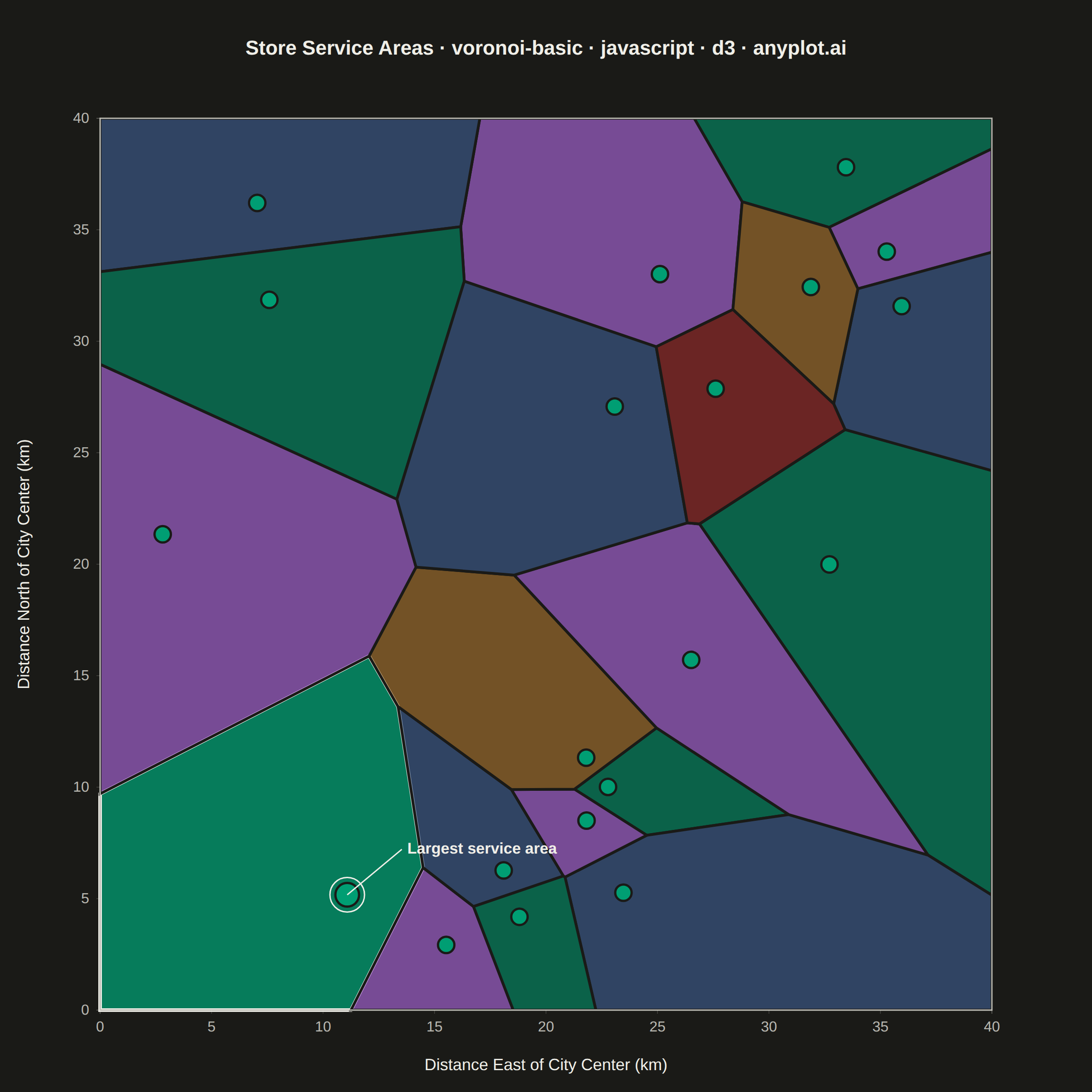
A Voronoi diagram partitions a plane into regions based on the distance to a set of seed points, where each region contains all points closer to its seed than to any other. This visualization is essential for understanding spatial relationships, proximity analysis, and territorial boundaries. It reveals natural clustering patterns and helps identify areas of influence around data points.
// anyplot.ai
// voronoi-basic: Voronoi Diagram for Spatial Partitioning
// Library: d3 7.9.0 | JavaScript 22.23.2
// Quality: 93/100 | Created: 2026-09-02

//# anyplot-orientation: square
const t = window.ANYPLOT_TOKENS;
const { width, height } = window.ANYPLOT_SIZE;

// --- Data (in-memory, deterministic) ----------------------------------------
// Retail-store service areas across a metro grid, in km from the city center.
// A tiny fixed-seed LCG stands in for Math.random() (not reproducible in-browser).
function lcg(seed) {
  let s = seed;
  return () => {
    s = (s * 1664525 + 1013904223) % 4294967296;
    return s / 4294967296;
  };
}
const rand = lcg(42);
const N_STORES = 20;
const DOMAIN_MIN = 0;
const DOMAIN_MAX = 40;
const stores = Array.from({ length: N_STORES }, (_, i) => ({
  label: `Store ${i + 1}`,
  x: DOMAIN_MIN + 2 + rand() * (DOMAIN_MAX - DOMAIN_MIN - 4),
  y: DOMAIN_MIN + 2 + rand() * (DOMAIN_MAX - DOMAIN_MIN - 4),
}));

// --- Layout — symmetric margins keep the plot area a true square, so the
// Voronoi cells (computed directly in pixel space below) aren't stretched. ---
const margin = { top: 130, right: 110, bottom: 90, left: 110 };
const iw = width - margin.left - margin.right;
const ih = height - margin.top - margin.bottom;

const xScale = d3.scaleLinear().domain([DOMAIN_MIN, DOMAIN_MAX]).range([0, iw]);
const yScale = d3.scaleLinear().domain([DOMAIN_MIN, DOMAIN_MAX]).range([ih, 0]);

// --- Voronoi tessellation, clipped to the visible plot bounding box ---------
const pixelPoints = stores.map((d) => [xScale(d.x), yScale(d.y)]);
const delaunay = d3.Delaunay.from(pixelPoints);
const voronoi = delaunay.voronoi([0, 0, iw, ih]);

// Greedy graph coloring over the Delaunay adjacency so neighboring cells never
// share a color — a more legible variant than cycling palette index by array order.
const colorIndex = new Array(N_STORES).fill(0);
for (let i = 0; i < N_STORES; i++) {
  const used = new Set();
  for (const j of delaunay.neighbors(i)) {
    if (j < i) used.add(colorIndex[j]);
  }
  let c = 0;
  while (used.has(c)) c++;
  colorIndex[i] = c % t.palette.length;
}

// Focal store — the one with the largest service area — gives the viewer a
// concrete entry point into the tessellation instead of uniform visual weight.
const cellAreas = stores.map((_, i) => Math.abs(d3.polygonArea(voronoi.cellPolygon(i))));
const focalIndex = d3.greatestIndex(cellAreas);

// --- SVG mount ----------------------------------------------------------------
const svg = d3.select("#container").append("svg").attr("width", width).attr("height", height);
const g = svg.append("g").attr("transform", `translate(${margin.left},${margin.top})`);

// --- Voronoi cells --------------------------------------------------------------
// The focal cell (largest service area) gets a touch more fill opacity and a
// heavier ink-toned border so it reads as the entry point into the tessellation.
g.append("g")
  .selectAll("path")
  .data(
    stores.map((d, i) => ({
      path: voronoi.renderCell(i),
      color: t.palette[colorIndex[i]],
      focal: i === focalIndex,
    }))
  )
  .join("path")
  .attr("d", (d) => d.path)
  .attr("fill", (d) => d.color)
  .attr("fill-opacity", (d) => (d.focal ? 0.75 : 0.55))
  .attr("stroke", (d) => (d.focal ? t.ink : t.pageBg))
  .attr("stroke-width", (d) => (d.focal ? 4 : 3));

// --- Bounding box outline -------------------------------------------------------
g.append("rect")
  .attr("x", 0)
  .attr("y", 0)
  .attr("width", iw)
  .attr("height", ih)
  .attr("fill", "none")
  .attr("stroke", t.inkSoft)
  .attr("stroke-width", 1.5);

// --- Axes ---------------------------------------------------------------------
// Restrained treatment (short ticks, thin low-contrast domain line) so the
// tessellation's cell colors stay the primary content, not the chrome.
const xAxis = g
  .append("g")
  .attr("transform", `translate(0,${ih})`)
  .call(d3.axisBottom(xScale).ticks(8).tickSize(4).tickPadding(8));
const yAxis = g.append("g").call(d3.axisLeft(yScale).ticks(8).tickSize(4).tickPadding(8));
for (const ax of [xAxis, yAxis]) {
  ax.selectAll("text").attr("fill", t.inkSoft).style("font-size", "16px");
  ax.selectAll("line").attr("stroke", t.grid).attr("stroke-width", 1);
  ax.select(".domain").attr("stroke", t.grid).attr("stroke-width", 1);
}

g.append("text")
  .attr("x", iw / 2)
  .attr("y", ih + 66)
  .attr("text-anchor", "middle")
  .attr("fill", t.ink)
  .style("font-size", "18px")
  .text("Distance East of City Center (km)");

g.append("text")
  .attr("transform", "rotate(-90)")
  .attr("x", -ih / 2)
  .attr("y", -78)
  .attr("text-anchor", "middle")
  .attr("fill", t.ink)
  .style("font-size", "18px")
  .text("Distance North of City Center (km)");

// --- Seed points — the store locations, marked prominently in brand green ---
// The focal store (largest service area) gets a larger marker and an outer
// ring so it doubles as the entry point the callout label points to.
g.append("g")
  .selectAll("circle")
  .data(pixelPoints.map((d, i) => ({ d, focal: i === focalIndex })))
  .join("circle")
  .attr("cx", (d) => d.d[0])
  .attr("cy", (d) => d.d[1])
  .attr("r", (d) => (d.focal ? 13 : 9))
  .attr("fill", t.palette[0])
  .attr("stroke", t.pageBg)
  .attr("stroke-width", 2.5);

g.append("circle")
  .attr("cx", pixelPoints[focalIndex][0])
  .attr("cy", pixelPoints[focalIndex][1])
  .attr("r", 19)
  .attr("fill", "none")
  .attr("stroke", t.ink)
  .attr("stroke-width", 1.5);

// --- Focal callout — leader line + label pointing at the largest service area,
// anchored so it always points away from the canvas edges it's nearest to. ---
const focalPx = pixelPoints[focalIndex];
const dirX = focalPx[0] > iw / 2 ? -1 : 1;
const dirY = focalPx[1] > ih / 2 ? -1 : 1;
const calloutX = focalPx[0] + dirX * 60;
const calloutY = focalPx[1] + dirY * 50;
g.append("line")
  .attr("x1", focalPx[0])
  .attr("y1", focalPx[1])
  .attr("x2", calloutX)
  .attr("y2", calloutY)
  .attr("stroke", t.ink)
  .attr("stroke-width", 1.5);
g.append("text")
  .attr("x", calloutX + dirX * 6)
  .attr("y", calloutY)
  .attr("text-anchor", dirX > 0 ? "start" : "end")
  .attr("dominant-baseline", "middle")
  .attr("fill", t.ink)
  .style("font-size", "17px")
  .style("font-weight", "600")
  .text("Largest service area");

// --- Title --------------------------------------------------------------------
const titleText = "Store Service Areas · voronoi-basic · javascript · d3 · anyplot.ai";
const titleFontSize = titleText.length > 67 ? Math.round(22 * (67 / titleText.length)) : 22;
svg
  .append("text")
  .attr("x", width / 2)
  .attr("y", 60)
  .attr("text-anchor", "middle")
  .attr("fill", t.ink)
  .style("font-size", `${titleFontSize}px`)
  .style("font-weight", "600")
  .text(titleText);
Runnable source as JSON, for any HTTP client: https://api.anyplot.ai/specs/voronoi-basic/d3/code. Any spec id and library id listed in llms-full.txt fit the same URL shape; every URL below is complete and callable.
{
  "spec_id": "voronoi-basic",
  "language": "javascript",
  "library": "d3",
  "page": "https://anyplot.ai/voronoi-basic/javascript/d3",
  "hub": "https://anyplot.ai/voronoi-basic",
  "code_json": "https://api.anyplot.ai/specs/voronoi-basic/d3/code",
  "spec_json": "https://api.anyplot.ai/specs/voronoi-basic",
  "render_light_png": "https://storage.googleapis.com/anyplot-images/plots/voronoi-basic/javascript/d3/plot-light.png",
  "render_dark_png": "https://storage.googleapis.com/anyplot-images/plots/voronoi-basic/javascript/d3/plot-dark.png",
  "interactive_light_html": "https://storage.googleapis.com/anyplot-images/plots/voronoi-basic/javascript/d3/plot-light.html",
  "interactive_dark_html": "https://storage.googleapis.com/anyplot-images/plots/voronoi-basic/javascript/d3/plot-dark.html",
  "quality_score": 93.0,
  "license": "MIT",
  "guide": "https://anyplot.ai/llms.txt"
}
Part of Voronoi Diagram for Spatial Partitioning on anyplot.ai.