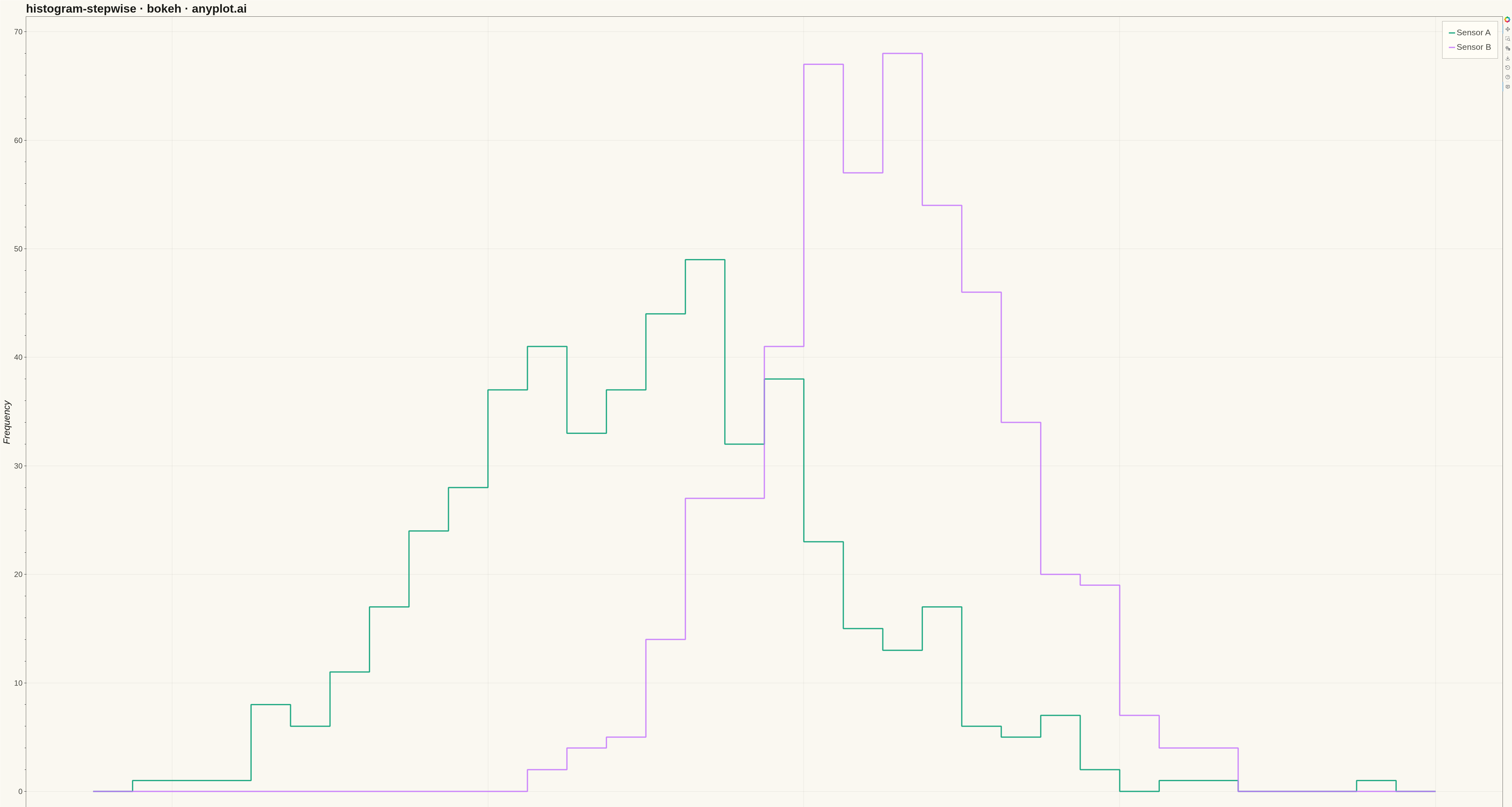
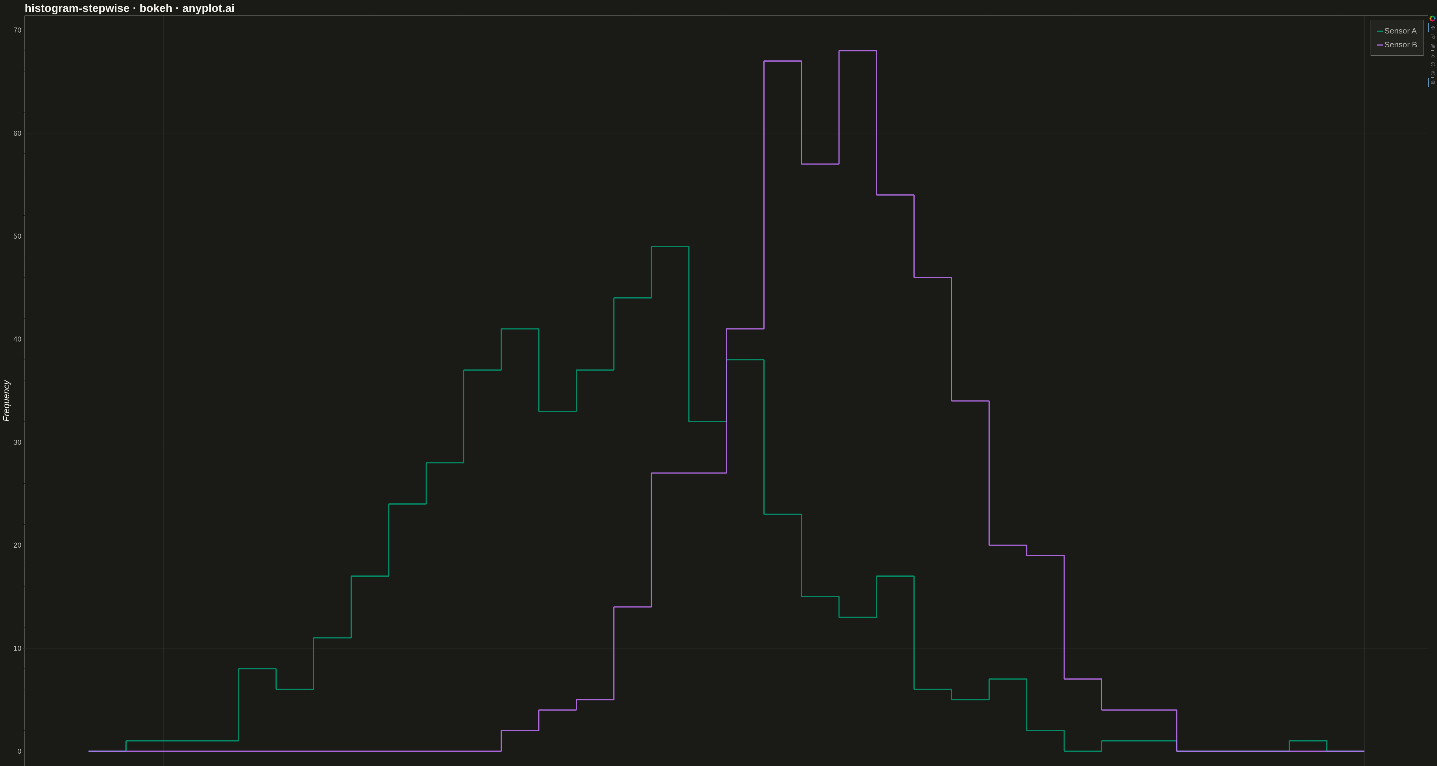
A histogram displayed as step lines (outline only) without filled bars. The distribution is shown as connected horizontal and vertical line segments, creating a step function appearance.
""" anyplot.ai
histogram-stepwise: Step Histogram
Library: bokeh 3.9.0 | Python 3.13.13
Quality: 96/100 | Updated: 2026-05-12
"""

import os
import sys
import time
from pathlib import Path

# Remove the script's directory from sys.path to avoid circular import
sys.path = [p for p in sys.path if not p.endswith("python")]

import numpy as np
from bokeh.io import output_file, save
from bokeh.models import HoverTool
from bokeh.plotting import figure
from selenium import webdriver
from selenium.webdriver.chrome.options import Options

# Theme tokens
THEME = os.getenv("ANYPLOT_THEME", "light")
PAGE_BG = "#FAF8F1" if THEME == "light" else "#1A1A17"
ELEVATED_BG = "#FFFDF6" if THEME == "light" else "#242420"
INK = "#1A1A17" if THEME == "light" else "#F0EFE8"
INK_SOFT = "#4A4A44" if THEME == "light" else "#B8B7B0"

# Okabe-Ito palette (first series is always #009E73)
IMPRINT = ["#009E73", "#C475FD", "#4467A3", "#BD8233", "#AE3030", "#2ABCCD", "#954477"]

# Data - Two distributions with different spreads for comparison
np.random.seed(42)
data1 = np.random.normal(loc=50, scale=12, size=500)  # Temperature sensor A
data2 = np.random.normal(loc=65, scale=8, size=500)  # Temperature sensor B (tighter spread)

# Compute histogram bins and counts
bins = np.linspace(15, 100, 35)
counts1, edges1 = np.histogram(data1, bins=bins)
counts2, edges2 = np.histogram(data2, bins=bins)

# Create step coordinates for step histogram (outline only)
x1 = np.repeat(edges1, 2)[1:-1]
y1 = np.repeat(counts1, 2)
x2 = np.repeat(edges2, 2)[1:-1]
y2 = np.repeat(counts2, 2)

# Create figure
p = figure(
    width=4800,
    height=2700,
    title="histogram-stepwise · bokeh · anyplot.ai",
    x_axis_label="Temperature (°C)",
    y_axis_label="Frequency",
    toolbar_location="right",
)

# Plot step histograms with Okabe-Ito colors
line1 = p.line(x1, y1, line_width=4, color=IMPRINT[0], legend_label="Sensor A", alpha=0.85)
line2 = p.line(x2, y2, line_width=4, color=IMPRINT[1], legend_label="Sensor B", alpha=0.85)

# Add hover tooltips for interactivity
hover1 = HoverTool(renderers=[line1], tooltips=[("Temperature (°C)", "$x{0.0}"), ("Frequency", "$y{0}")])
hover2 = HoverTool(renderers=[line2], tooltips=[("Temperature (°C)", "$x{0.0}"), ("Frequency", "$y{0}")])
p.add_tools(hover1, hover2)

# Title styling
p.title.text_font_size = "28pt"
p.title.text_color = INK

# Axis label styling
p.xaxis.axis_label_text_font_size = "22pt"
p.yaxis.axis_label_text_font_size = "22pt"
p.xaxis.axis_label_text_color = INK
p.yaxis.axis_label_text_color = INK

# Tick label styling
p.xaxis.major_label_text_font_size = "18pt"
p.yaxis.major_label_text_font_size = "18pt"
p.xaxis.major_label_text_color = INK_SOFT
p.yaxis.major_label_text_color = INK_SOFT

# Grid styling (subtle)
p.xgrid.grid_line_color = INK
p.ygrid.grid_line_color = INK
p.xgrid.grid_line_alpha = 0.10
p.ygrid.grid_line_alpha = 0.10

# Axis and border styling
p.axis.axis_line_color = INK_SOFT
p.axis.major_tick_line_color = INK_SOFT
p.background_fill_color = PAGE_BG
p.border_fill_color = PAGE_BG
p.outline_line_color = INK_SOFT

# Legend styling (improved visibility)
p.legend.label_text_font_size = "20pt"
p.legend.label_text_color = INK_SOFT
p.legend.background_fill_color = ELEVATED_BG
p.legend.border_line_color = INK_SOFT
p.legend.location = "top_right"
p.legend.padding = 20
p.legend.spacing = 15
p.legend.margin = 15

# Save HTML
output_file(f"plot-{THEME}.html")
save(p)

# Screenshot with headless Chrome
W, H = 4800, 2700
opts = Options()
for arg in (
    "--headless=new",
    "--no-sandbox",
    "--disable-dev-shm-usage",
    "--disable-gpu",
    f"--window-size={W},{H}",
    "--hide-scrollbars",
):
    opts.add_argument(arg)
driver = webdriver.Chrome(options=opts)
driver.set_window_size(W, H)
driver.get(f"file://{Path(f'plot-{THEME}.html').resolve()}")
time.sleep(3)
driver.save_screenshot(f"plot-{THEME}.png")
driver.quit()
Runnable source as JSON, for any HTTP client: https://api.anyplot.ai/specs/histogram-stepwise/bokeh/code. Any spec id and library id listed in llms-full.txt fit the same URL shape; every URL below is complete and callable.
{
  "spec_id": "histogram-stepwise",
  "language": "python",
  "library": "bokeh",
  "page": "https://anyplot.ai/histogram-stepwise/python/bokeh",
  "hub": "https://anyplot.ai/histogram-stepwise",
  "code_json": "https://api.anyplot.ai/specs/histogram-stepwise/bokeh/code",
  "spec_json": "https://api.anyplot.ai/specs/histogram-stepwise",
  "render_light_png": "https://storage.googleapis.com/anyplot-images/plots/histogram-stepwise/python/bokeh/plot-light.png",
  "render_dark_png": "https://storage.googleapis.com/anyplot-images/plots/histogram-stepwise/python/bokeh/plot-dark.png",
  "interactive_light_html": "https://storage.googleapis.com/anyplot-images/plots/histogram-stepwise/python/bokeh/plot-light.html",
  "interactive_dark_html": "https://storage.googleapis.com/anyplot-images/plots/histogram-stepwise/python/bokeh/plot-dark.html",
  "quality_score": 96.0,
  "license": "MIT",
  "guide": "https://anyplot.ai/llms.txt"
}
Part of Step Histogram on anyplot.ai.