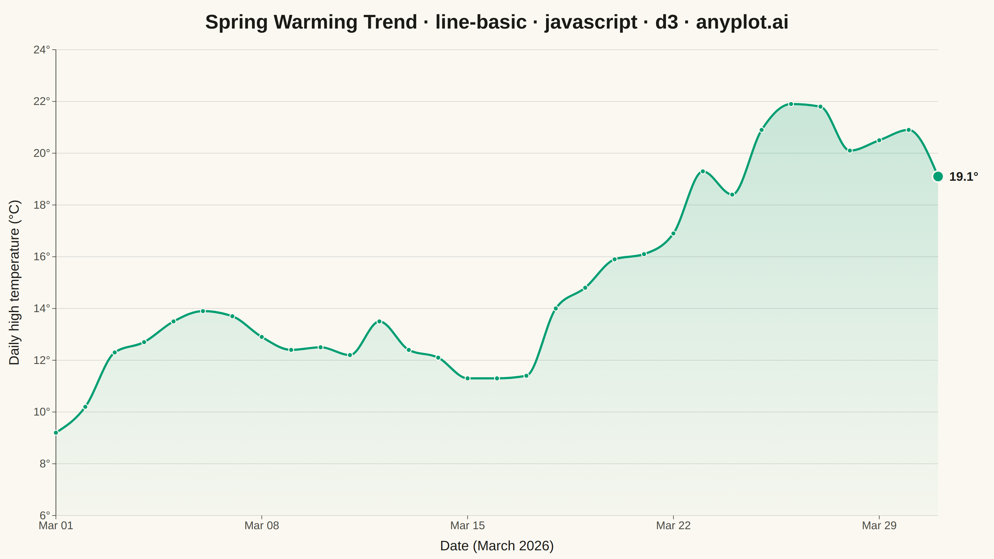
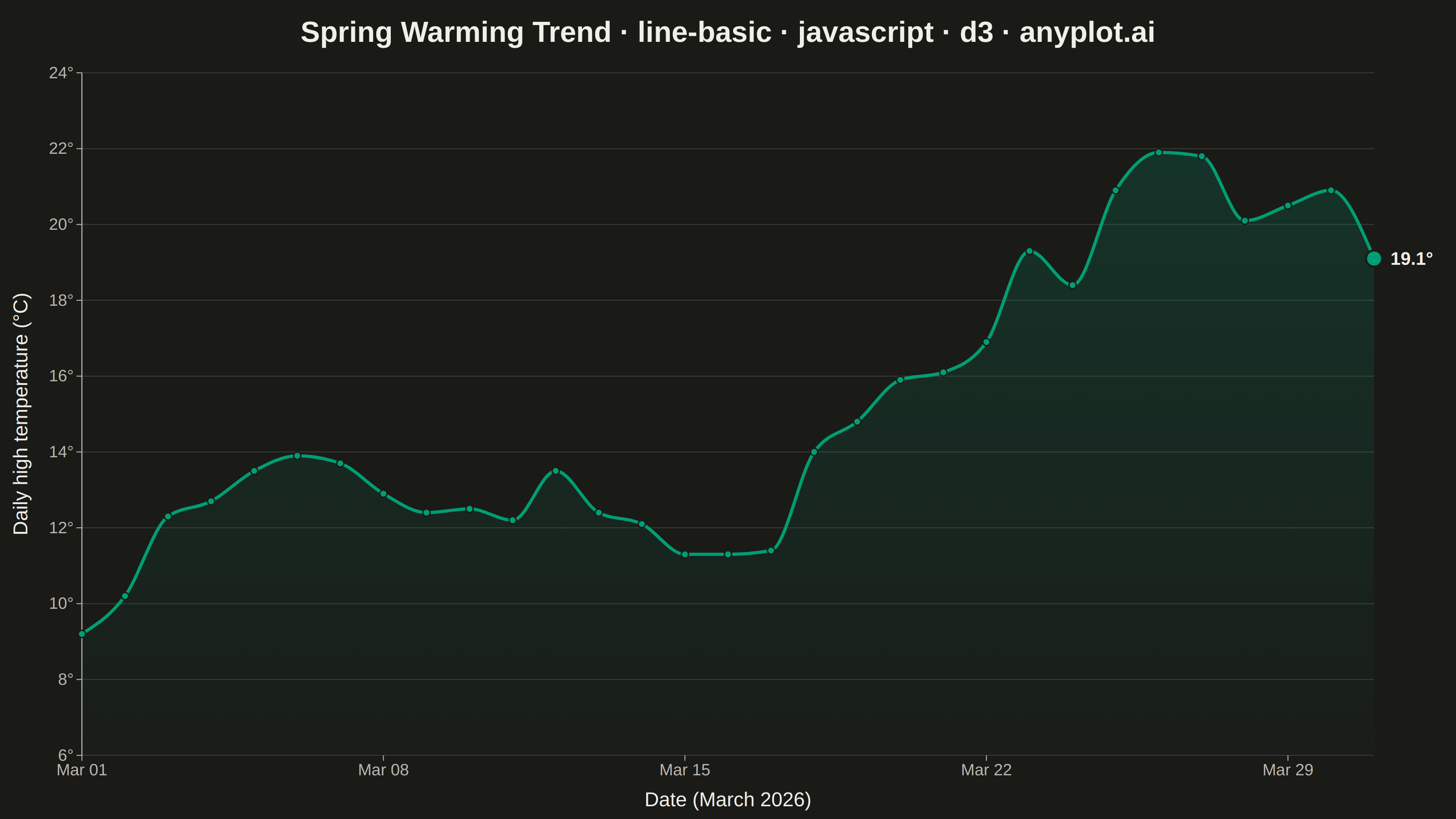
The same plot in 14 other libraries — JavaScript: Chart.js, Apache ECharts, Highcharts, MUI X Charts; Python: Altair, Bokeh, lets-plot, Matplotlib, Plotly, plotnine, Pygal, Seaborn; R: ggplot2; Julia: Makie.jl. Compare all 15 side by side: Basic Line Plot in Python, R, Julia and JavaScript.
A basic line plot connects data points with straight lines to show how a continuous variable changes over a sequence or time. It's ideal for revealing trends, patterns, and changes in data over ordered intervals. The simplicity of a single-line design makes it easy to interpret at a glance.
// anyplot.ai
// line-basic: Basic Line Plot
// Library: d3 7.9.0 | JavaScript 22.22.3
// Quality: 94/100 | Created: 2026-06-02
//# anyplot-orientation: landscape

const t = window.ANYPLOT_TOKENS;
const { width, height } = window.ANYPLOT_SIZE;
const margin = { top: 80, right: 90, bottom: 70, left: 90 };
const iw = width - margin.left - margin.right;
const ih = height - margin.top - margin.bottom;

// Data — daily high temperature (°C) for a spring month, deterministic LCG noise
const start = new Date(2026, 2, 1);
let seed = 42;
const rand = () => ((seed = (seed * 1103515245 + 12345) & 0x7fffffff) / 0x7fffffff);
const data = d3.range(31).map((i) => {
  const day = new Date(start);
  day.setDate(start.getDate() + i);
  const trend = 9 + (i / 30) * 11;
  const wobble = Math.sin(i / 3.2) * 2.6 + (rand() - 0.5) * 2.4;
  return { date: day, temp: +(trend + wobble).toFixed(1) };
});
const endpoint = data[data.length - 1];

// SVG mount
const svg = d3.select("#container").append("svg")
  .attr("width", width).attr("height", height);
const g = svg.append("g").attr("transform", `translate(${margin.left},${margin.top})`);

// Scales
const x = d3.scaleTime()
  .domain(d3.extent(data, (d) => d.date))
  .range([0, iw]);
const yMin = d3.min(data, (d) => d.temp);
const yMax = d3.max(data, (d) => d.temp);
const y = d3.scaleLinear()
  .domain([Math.floor(yMin - 2), Math.ceil(yMax + 2)])
  .nice()
  .range([ih, 0]);

// Vertical area-fill gradient — brand green, fading top->bottom
const defs = svg.append("defs");
const grad = defs.append("linearGradient")
  .attr("id", "fillGrad")
  .attr("gradientUnits", "userSpaceOnUse")
  .attr("x1", 0).attr("y1", 0).attr("x2", 0).attr("y2", ih);
grad.append("stop").attr("offset", "0%").attr("stop-color", t.palette[0]).attr("stop-opacity", 0.22);
grad.append("stop").attr("offset", "100%").attr("stop-color", t.palette[0]).attr("stop-opacity", 0.02);

// Gridlines (y-axis only, behind the data)
g.append("g")
  .attr("class", "grid")
  .call(d3.axisLeft(y).tickSize(-iw).tickFormat(""))
  .call((sel) => {
    sel.select(".domain").remove();
    sel.selectAll("line").attr("stroke", t.grid).attr("stroke-width", 1);
  });

// Axes — drop bottom domain spine for a lighter, more refined chrome
const xAxis = g.append("g")
  .attr("transform", `translate(0,${ih})`)
  .call(
    d3.axisBottom(x)
      .ticks(d3.timeWeek.every(1))
      .tickFormat(d3.timeFormat("%b %d"))
      .tickSizeOuter(0),
  );
const yAxis = g.append("g")
  .call(d3.axisLeft(y).ticks(7).tickFormat((d) => `${d}°`).tickSizeOuter(0));

for (const ax of [xAxis, yAxis]) {
  ax.selectAll("text").attr("fill", t.inkSoft).style("font-size", "18px");
  ax.selectAll(".tick line").attr("stroke", t.inkSoft);
}
xAxis.select(".domain").remove();
yAxis.select(".domain").attr("stroke", t.inkSoft).attr("stroke-width", 1.2);

// Axis labels
g.append("text")
  .attr("x", iw / 2).attr("y", ih + 56)
  .attr("text-anchor", "middle")
  .attr("fill", t.ink).style("font-size", "22px")
  .text("Date (March 2026)");
g.append("text")
  .attr("transform", "rotate(-90)")
  .attr("x", -ih / 2).attr("y", -60)
  .attr("text-anchor", "middle")
  .attr("fill", t.ink).style("font-size", "22px")
  .text("Daily high temperature (°C)");

// Area + line — first categorical series is Imprint palette[0]
const area = d3.area()
  .x((d) => x(d.date))
  .y0(ih)
  .y1((d) => y(d.temp))
  .curve(d3.curveMonotoneX);

const line = d3.line()
  .x((d) => x(d.date))
  .y((d) => y(d.temp))
  .curve(d3.curveMonotoneX);

g.append("path")
  .datum(data)
  .attr("fill", "url(#fillGrad)")
  .attr("d", area);

g.append("path")
  .datum(data)
  .attr("fill", "none")
  .attr("stroke", t.palette[0])
  .attr("stroke-width", 3.5)
  .attr("stroke-linecap", "round")
  .attr("stroke-linejoin", "round")
  .attr("d", line);

// Interior markers (skip the endpoint — emphasized separately below)
g.selectAll("circle.point")
  .data(data.slice(0, -1)).join("circle")
  .attr("class", "point")
  .attr("cx", (d) => x(d.date))
  .attr("cy", (d) => y(d.temp))
  .attr("r", 4)
  .attr("fill", t.palette[0])
  .attr("stroke", t.pageBg)
  .attr("stroke-width", 1.5);

// Emphasized endpoint marker + value label — narrative anchor for the warming trend
g.append("circle")
  .attr("cx", x(endpoint.date)).attr("cy", y(endpoint.temp))
  .attr("r", 9)
  .attr("fill", t.palette[0])
  .attr("stroke", t.pageBg)
  .attr("stroke-width", 2.5);

g.append("text")
  .attr("x", x(endpoint.date) + 18).attr("y", y(endpoint.temp))
  .attr("dy", "0.35em")
  .attr("text-anchor", "start")
  .attr("fill", t.ink)
  .style("font-size", "20px")
  .style("font-weight", "600")
  .text(`${endpoint.temp.toFixed(1)}°`);

// Title
svg.append("text")
  .attr("x", width / 2).attr("y", 46)
  .attr("text-anchor", "middle")
  .attr("fill", t.ink)
  .style("font-size", "32px")
  .style("font-weight", "600")
  .text("Spring Warming Trend · line-basic · javascript · d3 · anyplot.ai");
Runnable source as JSON, for any HTTP client: https://api.anyplot.ai/specs/line-basic/d3/code. Any spec id and library id listed in llms-full.txt fit the same URL shape; every URL below is complete and callable.
{
  "spec_id": "line-basic",
  "language": "javascript",
  "library": "d3",
  "page": "https://anyplot.ai/line-basic/javascript/d3",
  "hub": "https://anyplot.ai/line-basic",
  "code_json": "https://api.anyplot.ai/specs/line-basic/d3/code",
  "spec_json": "https://api.anyplot.ai/specs/line-basic",
  "render_light_png": "https://storage.googleapis.com/anyplot-images/plots/line-basic/javascript/d3/plot-light.png",
  "render_dark_png": "https://storage.googleapis.com/anyplot-images/plots/line-basic/javascript/d3/plot-dark.png",
  "interactive_light_html": "https://storage.googleapis.com/anyplot-images/plots/line-basic/javascript/d3/plot-light.html",
  "interactive_dark_html": "https://storage.googleapis.com/anyplot-images/plots/line-basic/javascript/d3/plot-dark.html",
  "quality_score": 94.0,
  "license": "MIT",
  "guide": "https://anyplot.ai/llms.txt"
}
Part of Basic Line Plot on anyplot.ai.