The same plot in 14 other libraries — Python: Altair, Bokeh, lets-plot, Matplotlib, Plotly, plotnine, Pygal, Seaborn; Julia: Makie.jl; JavaScript: Chart.js, D3.js, Apache ECharts, Highcharts, MUI X Charts. Compare all 15 side by side: PCA Biplot with Scores and Loading Vectors in Python, R, Julia and JavaScript.
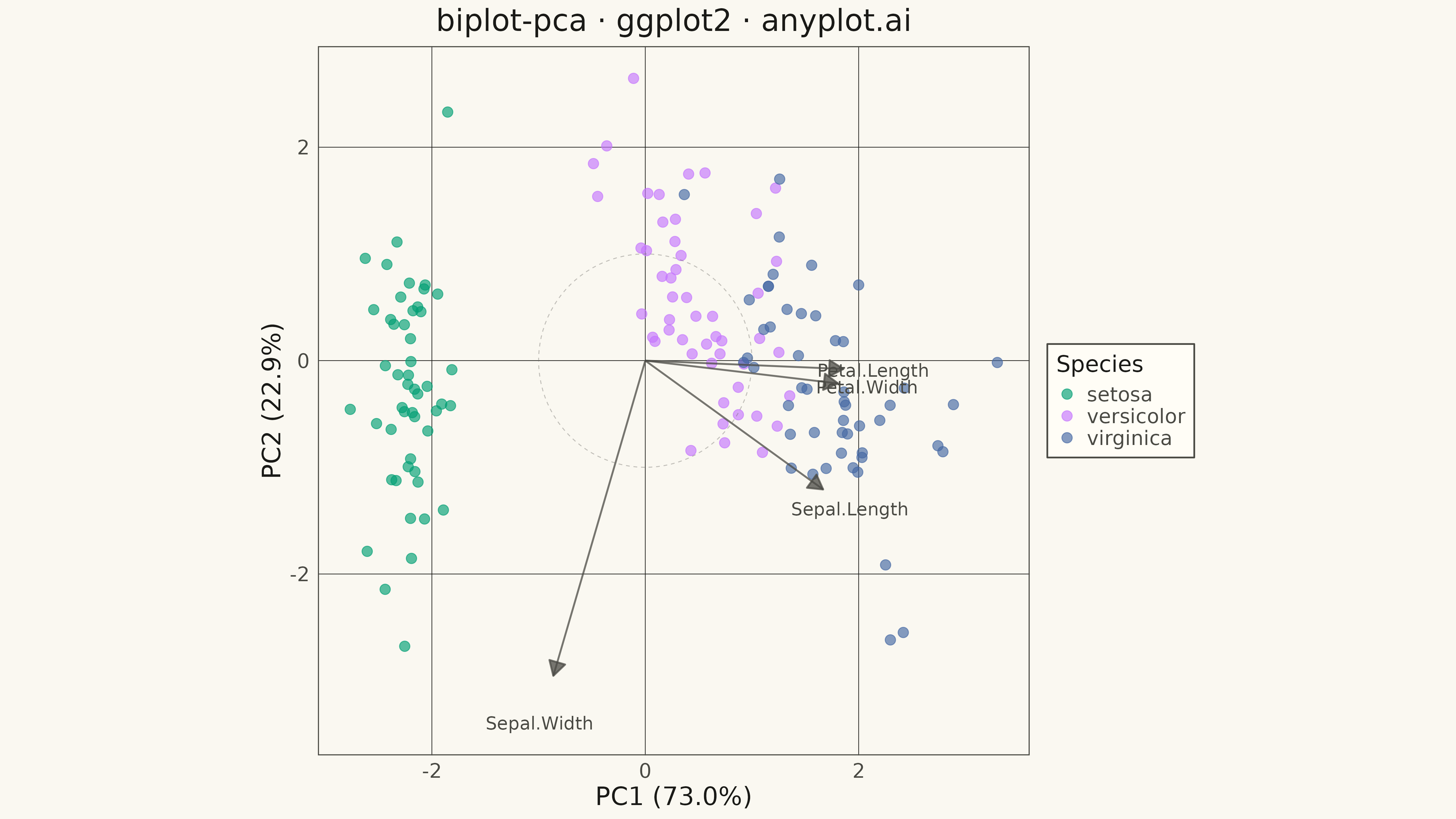
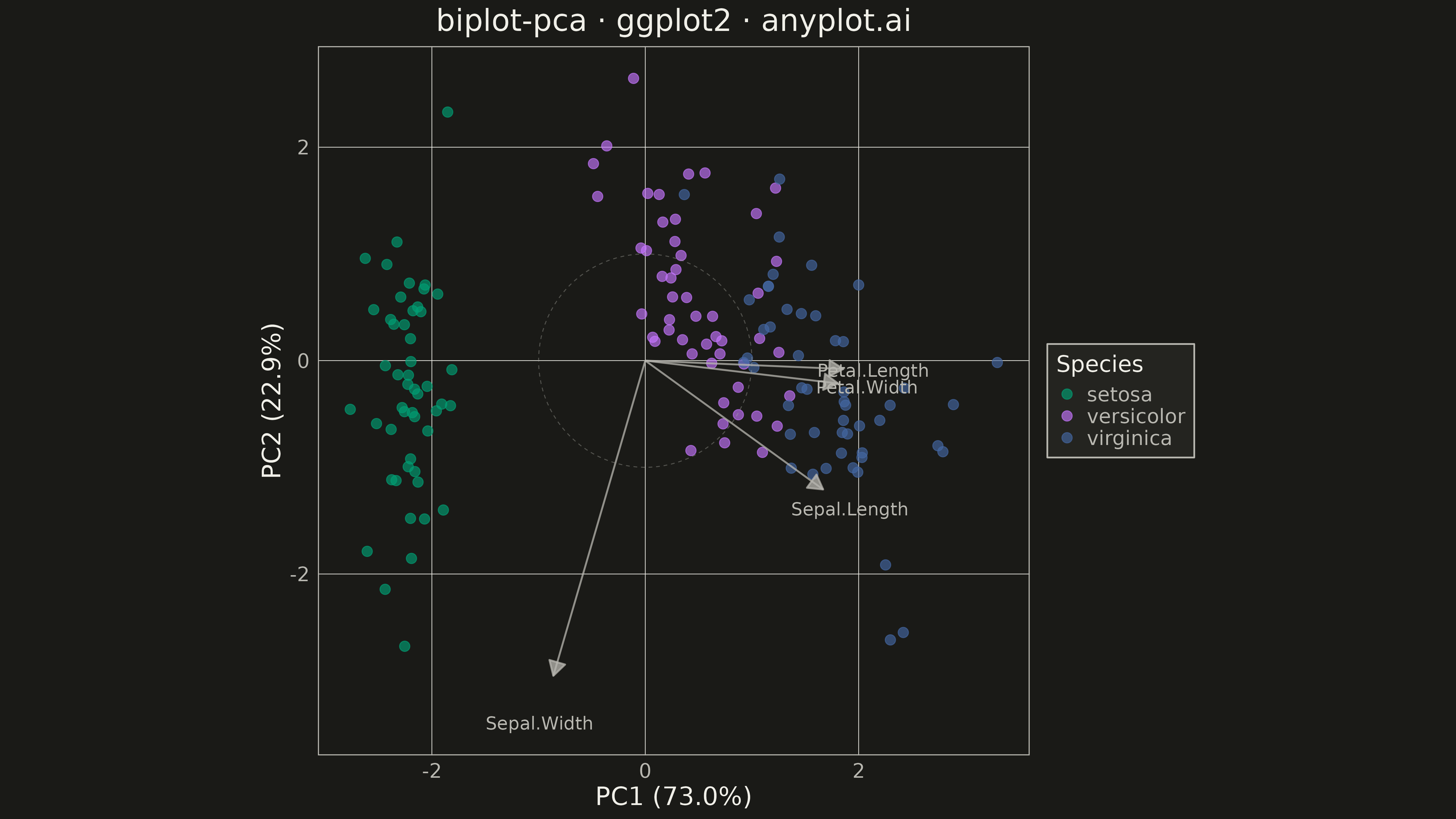
A PCA biplot simultaneously displays both observation scores (as points) and variable loadings (as arrows) in the principal component space. This dual representation is essential for interpreting PCA results, revealing how observations relate to each other and which original variables drive the separation along each principal component. The length and direction of loading arrows indicate variable importance and correlation with the components.
#' anyplot.ai
#' biplot-pca: PCA Biplot with Scores and Loading Vectors
#' Library: ggplot2 3.5.1 | R 4.4.1
#' Quality: 97/100 | Created: 2026-05-17

library(ggplot2)
library(dplyr)
library(scales)
library(ragg)

set.seed(42)

# --- Theme tokens ----
THEME       <- Sys.getenv("ANYPLOT_THEME", "light")
PAGE_BG     <- if (THEME == "light") "#FAF8F1" else "#1A1A17"
ELEVATED_BG <- if (THEME == "light") "#FFFDF6" else "#242420"
INK         <- if (THEME == "light") "#1A1A17" else "#F0EFE8"
INK_SOFT    <- if (THEME == "light") "#4A4A44" else "#B8B7B0"
INK_MUTED   <- if (THEME == "light") "#6B6A63" else "#A8A79F"
IMPRINT   <- c("#009E73", "#C475FD", "#4467A3", "#BD8233",
                 "#AE3030", "#2ABCCD", "#954477")

# --- Data: Perform PCA on iris dataset ----
pca_result <- prcomp(iris[, 1:4], scale. = TRUE)

# Extract and format scores
pca_scores <- as.data.frame(pca_result$x[, 1:2])
pca_scores$species <- iris$Species

# Extract variance explained (as percentages)
var_explained <- summary(pca_result)$importance[2, 1:2] * 100

# Extract and format loadings
loadings <- as.data.frame(pca_result$rotation[, 1:2])
loadings$variable <- rownames(pca_result$rotation)

# Scale loadings for visibility alongside score points
loadings_scaled <- loadings
loadings_scaled$PC1 <- loadings_scaled$PC1 * 3.2
loadings_scaled$PC2 <- loadings_scaled$PC2 * 3.2

# --- Custom theme ----
anyplot_theme <- theme_minimal(base_size = 14) +
  theme(
    plot.background   = element_rect(fill = PAGE_BG, color = PAGE_BG),
    panel.background  = element_rect(fill = PAGE_BG, color = NA),
    panel.grid.major  = element_line(color = INK, linewidth = 0.25),
    panel.grid.minor  = element_blank(),
    axis.title        = element_text(color = INK, size = 20),
    axis.text         = element_text(color = INK_SOFT, size = 16),
    plot.title        = element_text(color = INK, size = 24, hjust = 0.5),
    legend.background = element_rect(fill = ELEVATED_BG, color = INK_SOFT),
    legend.text       = element_text(color = INK_SOFT, size = 16),
    legend.title      = element_text(color = INK, size = 18),
    panel.border      = element_rect(color = INK_SOFT, fill = NA, linewidth = 0.8)
  )

# --- Plot ----
p <- ggplot() +
  # Observation scores as points
  geom_point(
    data = pca_scores,
    aes(x = PC1, y = PC2, color = species),
    size = 3.5,
    alpha = 0.65
  ) +
  # Loading vectors as arrows from origin
  geom_segment(
    data = loadings_scaled,
    aes(x = 0, y = 0, xend = PC1, yend = PC2),
    arrow = arrow(length = unit(0.18, "inches"), type = "closed"),
    color = INK_SOFT,
    linewidth = 0.7,
    alpha = 0.75
  ) +
  # Variable labels on loading arrows
  geom_text(
    data = loadings_scaled,
    aes(x = PC1 * 1.15, y = PC2 * 1.15, label = variable),
    color = INK_SOFT,
    size = 5,
    fontface = "italic"
  ) +
  # Reference circle (unit circle for correlation scaling)
  annotate(
    "path",
    x = cos(seq(0, 2*pi, length.out = 100)),
    y = sin(seq(0, 2*pi, length.out = 100)),
    color = INK_MUTED,
    linewidth = 0.35,
    alpha = 0.4,
    linetype = "dashed"
  ) +
  # Color scale: species (first group uses #009E73)
  scale_color_manual(
    values = c(
      "setosa" = IMPRINT[1],
      "versicolor" = IMPRINT[2],
      "virginica" = IMPRINT[3]
    ),
    name = "Species"
  ) +
  # Labels with variance explained
  labs(
    title = "biplot-pca · ggplot2 · anyplot.ai",
    x = sprintf("PC1 (%.1f%%)", var_explained[1]),
    y = sprintf("PC2 (%.1f%%)", var_explained[2])
  ) +
  # Equal aspect ratio for visual fairness
  coord_fixed() +
  anyplot_theme

# --- Save ----
ggsave(
  filename = sprintf("plot-%s.png", THEME),
  plot = p,
  device = ragg::agg_png,
  width = 16,
  height = 9,
  units = "in",
  dpi = 300
)
Runnable source as JSON, for any HTTP client: https://api.anyplot.ai/specs/biplot-pca/ggplot2/code. Any spec id and library id listed in llms-full.txt fit the same URL shape; every URL below is complete and callable.
{
  "spec_id": "biplot-pca",
  "language": "r",
  "library": "ggplot2",
  "page": "https://anyplot.ai/biplot-pca/r/ggplot2",
  "hub": "https://anyplot.ai/biplot-pca",
  "code_json": "https://api.anyplot.ai/specs/biplot-pca/ggplot2/code",
  "spec_json": "https://api.anyplot.ai/specs/biplot-pca",
  "render_light_png": "https://storage.googleapis.com/anyplot-images/plots/biplot-pca/r/ggplot2/plot-light.png",
  "render_dark_png": "https://storage.googleapis.com/anyplot-images/plots/biplot-pca/r/ggplot2/plot-dark.png",
  "quality_score": 97.0,
  "license": "MIT",
  "guide": "https://anyplot.ai/llms.txt"
}
Part of PCA Biplot with Scores and Loading Vectors on anyplot.ai.