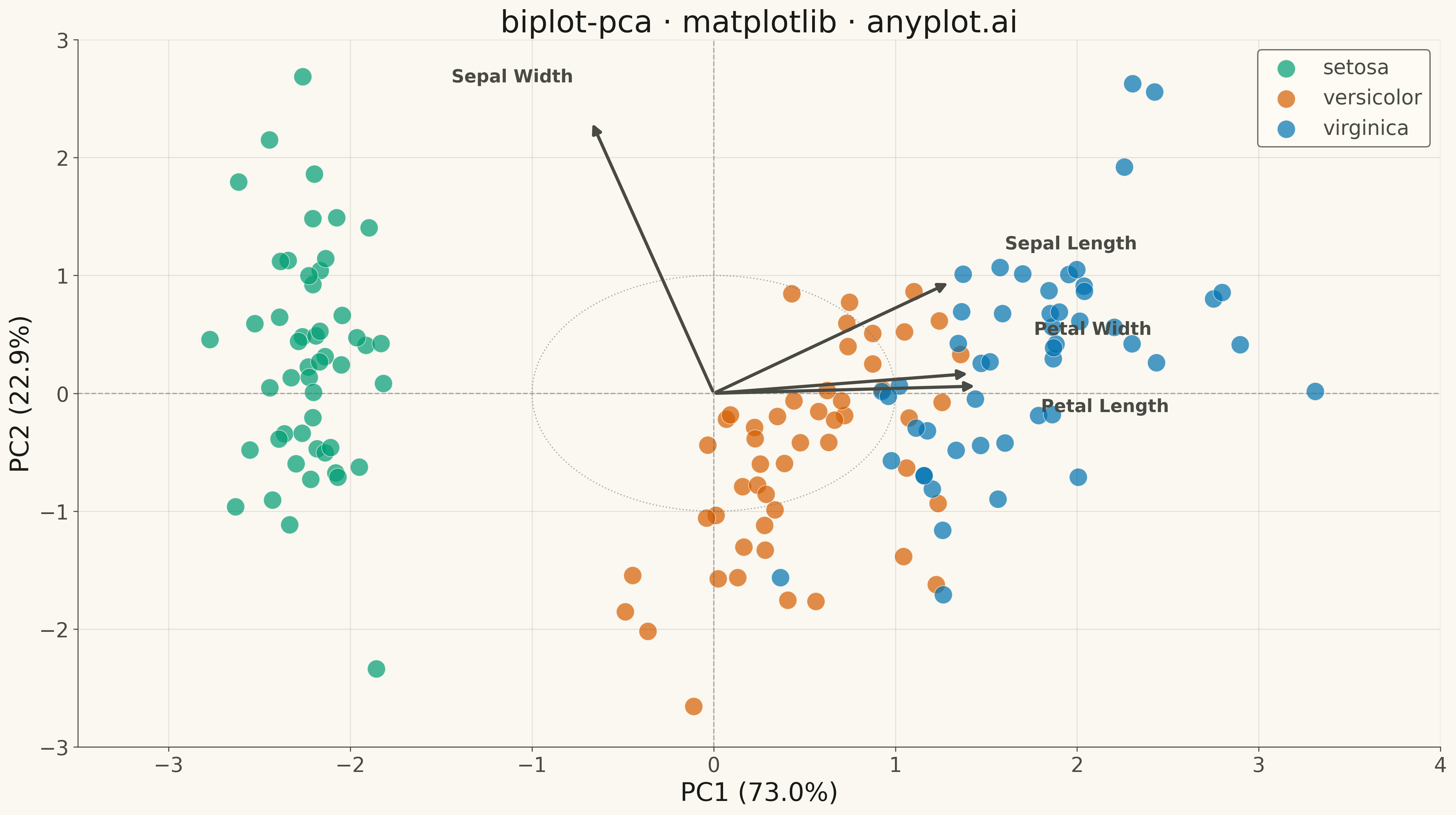
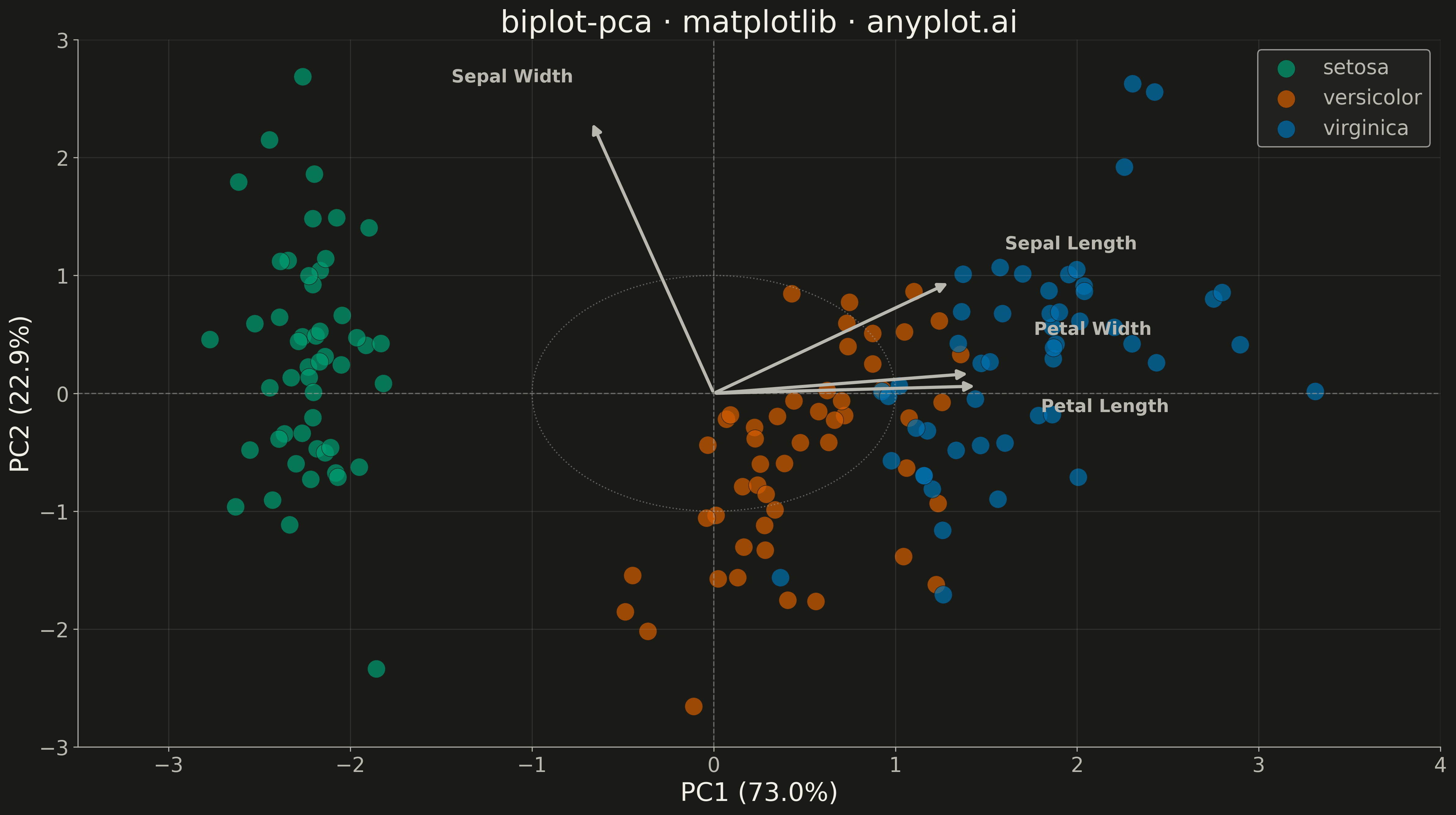
PCA Biplot with Scores and Loading Vectors — Matplotlib

A PCA biplot simultaneously displays both observation scores (as points) and variable loadings (as arrows) in the principal component space. This dual representation is essential for interpreting PCA results, revealing how observations relate to each other and which original variables drive the separation along each principal component. The length and direction of loading arrows indicate variable importance and correlation with the components.

PCA Biplot with Scores and Loading Vectors rendered with Matplotlib

Python source (Matplotlib)

""" anyplot.ai
biplot-pca: PCA Biplot with Scores and Loading Vectors
Library: matplotlib 3.10.9 | Python 3.13.13
Quality: 83/100 | Updated: 2026-05-17
"""

import matplotlib.pyplot as plt
from sklearn.datasets import load_iris
from sklearn.decomposition import PCA
from sklearn.preprocessing import StandardScaler


# Load and prepare data
iris = load_iris()
X = iris.data
y = iris.target
feature_names = ["Sepal Length", "Sepal Width", "Petal Length", "Petal Width"]
target_names = iris.target_names

# Standardize features
scaler = StandardScaler()
X_scaled = scaler.fit_transform(X)

# Perform PCA
pca = PCA(n_components=2)
scores = pca.fit_transform(X_scaled)
loadings = pca.components_.T  # Transpose to get (n_features, n_components)
explained_variance = pca.explained_variance_ratio_ * 100

# Create figure
fig, ax = plt.subplots(figsize=(16, 9))

# Define colors for each class
colors = ["#306998", "#FFD43B", "#E74C3C"]

# Plot observation scores (points) by group
for i, (target, color) in enumerate(zip(target_names, colors, strict=True)):
    mask = y == i
    ax.scatter(
        scores[mask, 0],
        scores[mask, 1],
        c=color,
        s=150,
        alpha=0.7,
        label=target.capitalize(),
        edgecolors="white",
        linewidth=0.5,
    )

# Scale loadings for visibility - use smaller scale to keep arrows within plot
scale_factor = 2.5

# Plot loading arrows and labels
arrow_color = "#2C3E50"
for i, feature in enumerate(feature_names):
    x_arrow = loadings[i, 0] * scale_factor
    y_arrow = loadings[i, 1] * scale_factor

    ax.annotate(
        "",
        xy=(x_arrow, y_arrow),
        xytext=(0, 0),
        arrowprops={"arrowstyle": "-|>", "color": arrow_color, "lw": 2.5, "mutation_scale": 15},
    )

    # Position text with custom offsets to avoid overlap
    # Manual adjustments for Iris dataset features
    offsets = {
        "Sepal Length": (0.3, 0.25),
        "Sepal Width": (-0.1, 0.3),
        "Petal Length": (0.35, -0.25),
        "Petal Width": (0.35, 0.3),
    }
    dx, dy = offsets.get(feature, (0.3, 0.3))
    text_x = x_arrow + dx
    text_y = y_arrow + dy

    # Adjust alignment based on position
    ha = "left" if x_arrow >= 0 else "right"
    va = "bottom" if y_arrow >= 0 else "top"

    ax.text(text_x, text_y, feature, fontsize=14, ha=ha, va=va, fontweight="bold", color=arrow_color)

# Draw reference lines at origin
ax.axhline(y=0, color="gray", linestyle="--", linewidth=1, alpha=0.5)
ax.axvline(x=0, color="gray", linestyle="--", linewidth=1, alpha=0.5)

# Labels and title
ax.set_xlabel(f"PC1 ({explained_variance[0]:.1f}%)", fontsize=20)
ax.set_ylabel(f"PC2 ({explained_variance[1]:.1f}%)", fontsize=20)
ax.set_title("biplot-pca · matplotlib · pyplots.ai", fontsize=24)

# Styling
ax.tick_params(axis="both", labelsize=16)
ax.legend(fontsize=16, loc="upper right", framealpha=0.9)
ax.grid(True, alpha=0.3, linestyle="--")

# Set axis limits with some padding
ax.set_xlim(-3.5, 4)
ax.set_ylim(-3, 3)

plt.tight_layout()
plt.savefig("plot.png", dpi=300, bbox_inches="tight")

Part of PCA Biplot with Scores and Loading Vectors on anyplot.ai.

PCA Biplot with Scores and Loading Vectors — Matplotlib

Python source (Matplotlib)

Other implementations