The same plot in 14 other libraries — JavaScript: D3.js, Apache ECharts, Highcharts, MUI X Charts; Python: Altair, Bokeh, lets-plot, Matplotlib, Plotly, plotnine, Pygal, Seaborn; R: ggplot2; Julia: Makie.jl. Compare all 15 side by side: PCA Biplot with Scores and Loading Vectors in Python, R, Julia and JavaScript.
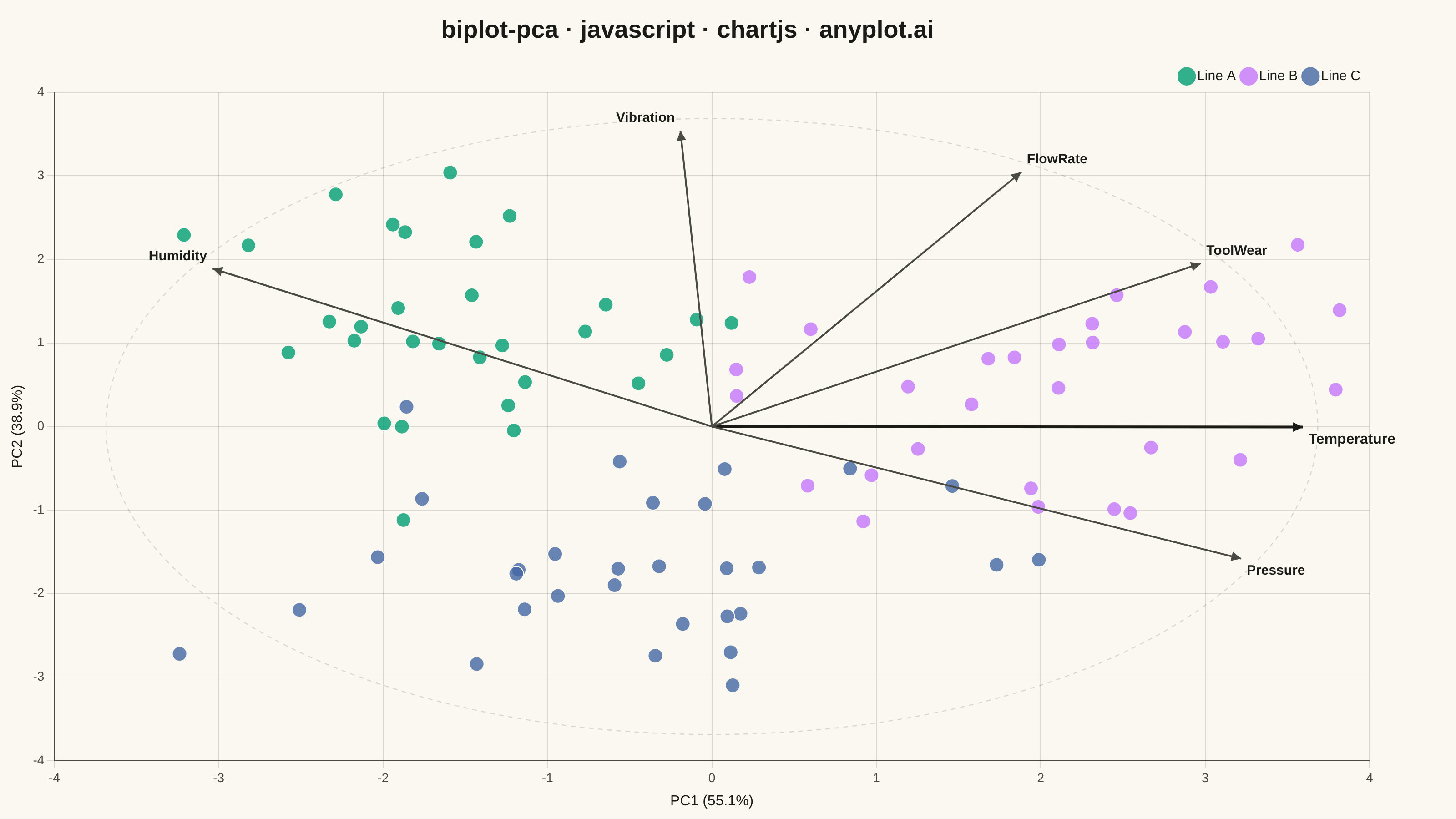
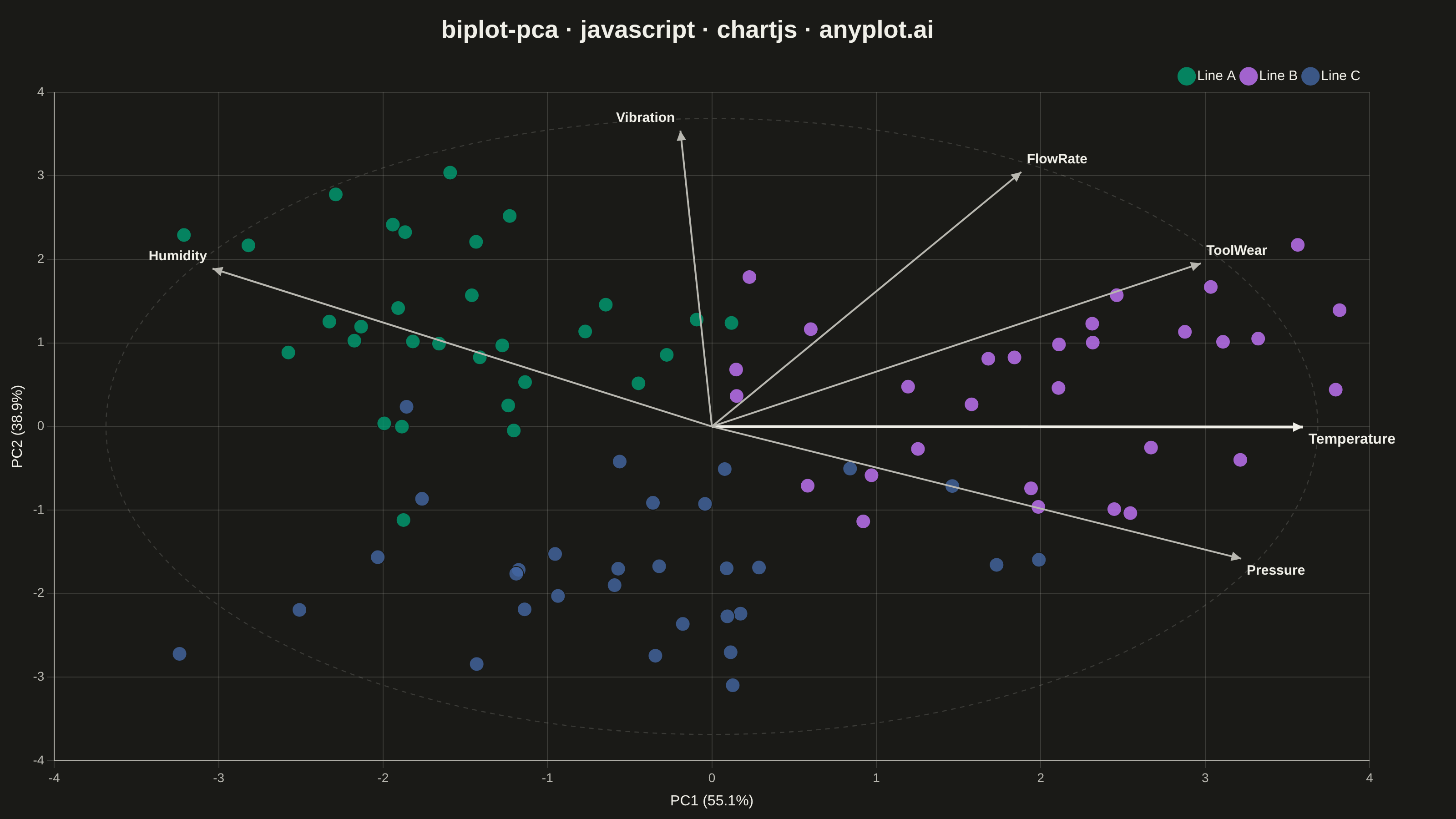
A PCA biplot simultaneously displays both observation scores (as points) and variable loadings (as arrows) in the principal component space. This dual representation is essential for interpreting PCA results, revealing how observations relate to each other and which original variables drive the separation along each principal component. The length and direction of loading arrows indicate variable importance and correlation with the components.
// anyplot.ai
// biplot-pca: PCA Biplot with Scores and Loading Vectors
// Library: chartjs 4.4.7 | JavaScript 22.23.2
// Quality: 92/100 | Created: 2026-09-01
//# anyplot-orientation: landscape

const t = window.ANYPLOT_TOKENS;

// --- Deterministic PRNG (LCG + Box-Muller) ----------------------------------
const lcg = (seed) => {
    let s = seed >>> 0;
    return () => {
        s = (Math.imul(1664525, s) + 1013904223) >>> 0;
        return s / 4294967296;
    };
};
const rand = lcg(42);
const randn = () => {
    const u1 = Math.max(rand(), 1e-9);
    const u2 = rand();
    return Math.sqrt(-2 * Math.log(u1)) * Math.cos(2 * Math.PI * u2);
};

// --- Data: process-monitoring measurements across three production lines ---
// Each observation is generated from a 2D latent process state (per-line
// offset + shared noise), so the six correlated measurements carry a real
// low-rank structure for PCA to recover.
const lines = ["Line A", "Line B", "Line C"];
const latentOffsets = [
    [-2.1, 1.1],
    [2.0, 1.0],
    [0.0, -2.2],
];
const nPerLine = 30;
const variables = ["Temperature", "Pressure", "Humidity", "FlowRate", "Vibration", "ToolWear"];
// [weight on latent1, weight on latent2] per variable
const weights = [
    [1.0, 0.2],
    [0.9, -0.3],
    [-0.8, 0.4],
    [0.3, 1.0],
    [-0.2, 0.9],
    [0.6, 0.6],
];
const noiseSigma = 0.6;

const groupIndex = [];
const X = [];
lines.forEach((_, g) => {
    const [m1, m2] = latentOffsets[g];
    for (let k = 0; k < nPerLine; k++) {
        const latent1 = m1 + randn();
        const latent2 = m2 + randn();
        const row = weights.map(([a, b]) => a * latent1 + b * latent2 + noiseSigma * randn());
        X.push(row);
        groupIndex.push(g);
    }
});
const n = X.length;
const p = variables.length;

// --- Standardize columns (mean 0, sd 1) -> correlation-based PCA -----------
const means = variables.map((_, j) => X.reduce((s, row) => s + row[j], 0) / n);
const sds = variables.map((_, j) =>
    Math.sqrt(X.reduce((s, row) => s + (row[j] - means[j]) ** 2, 0) / (n - 1))
);
const Xs = X.map((row) => row.map((v, j) => (v - means[j]) / sds[j]));

// --- Correlation matrix (p x p) ---------------------------------------------
const corr = Array.from({ length: p }, (_, i) =>
    Array.from({ length: p }, (_, j) => Xs.reduce((s, row) => s + row[i] * row[j], 0) / (n - 1))
);

// --- Jacobi eigenvalue algorithm for symmetric matrices ---------------------
const jacobiEigen = (matrix, size) => {
    const a = matrix.map((row) => row.slice());
    const v = Array.from({ length: size }, (_, i) =>
        Array.from({ length: size }, (_, j) => (i === j ? 1 : 0))
    );
    for (let sweep = 0; sweep < 100; sweep++) {
        let offDiag = 0;
        for (let i = 0; i < size; i++) {
            for (let j = i + 1; j < size; j++) offDiag += a[i][j] * a[i][j];
        }
        if (offDiag < 1e-12) break;
        for (let pi = 0; pi < size - 1; pi++) {
            for (let qi = pi + 1; qi < size; qi++) {
                if (Math.abs(a[pi][qi]) < 1e-14) continue;
                const theta = (a[qi][qi] - a[pi][pi]) / (2 * a[pi][qi]);
                const sign = theta >= 0 ? 1 : -1;
                const tVal = sign / (Math.abs(theta) + Math.sqrt(theta * theta + 1));
                const c = 1 / Math.sqrt(tVal * tVal + 1);
                const s = tVal * c;
                const app = a[pi][pi];
                const aqq = a[qi][qi];
                const apq = a[pi][qi];
                a[pi][pi] = c * c * app - 2 * s * c * apq + s * s * aqq;
                a[qi][qi] = s * s * app + 2 * s * c * apq + c * c * aqq;
                a[pi][qi] = 0;
                a[qi][pi] = 0;
                for (let i = 0; i < size; i++) {
                    if (i === pi || i === qi) continue;
                    const aip = a[i][pi];
                    const aiq = a[i][qi];
                    a[i][pi] = c * aip - s * aiq;
                    a[pi][i] = a[i][pi];
                    a[i][qi] = s * aip + c * aiq;
                    a[qi][i] = a[i][qi];
                }
                for (let i = 0; i < size; i++) {
                    const vip = v[i][pi];
                    const viq = v[i][qi];
                    v[i][pi] = c * vip - s * viq;
                    v[i][qi] = s * vip + c * viq;
                }
            }
        }
    }
    return { values: Array.from({ length: size }, (_, i) => a[i][i]), vectors: v };
};

const { values: eigVals, vectors: eigVecs } = jacobiEigen(corr, p);
const order = eigVals.map((_, i) => i).sort((i, j) => eigVals[j] - eigVals[i]);
const [pc1, pc2] = order;
const totalVar = eigVals.reduce((s, v) => s + v, 0);
const varExplained1 = (eigVals[pc1] / totalVar) * 100;
const varExplained2 = (eigVals[pc2] / totalVar) * 100;

// --- Scores: project standardized data onto the top two eigenvectors -------
const scores = Xs.map((row) => [
    row.reduce((s, v, j) => s + v * eigVecs[j][pc1], 0),
    row.reduce((s, v, j) => s + v * eigVecs[j][pc2], 0),
]);

// --- Correlation loadings: eigenvector scaled by sqrt(eigenvalue) ----------
// Each loading lies within the unit circle, representing the correlation
// between the original variable and the principal component.
const loadingsRaw = variables.map((_, j) => [
    eigVecs[j][pc1] * Math.sqrt(eigVals[pc1]),
    eigVecs[j][pc2] * Math.sqrt(eigVals[pc2]),
]);

// Scale loadings so arrow tips reach a comparable magnitude to the score
// cloud, per the spec's "scale loadings appropriately" guidance.
const scoreRadius = Math.max(...scores.map(([x, y]) => Math.sqrt(x * x + y * y)));
const loadingRadius = Math.max(...loadingsRaw.map(([x, y]) => Math.sqrt(x * x + y * y)));
const loadingScale = (scoreRadius / loadingRadius) * 0.85;
const loadings = loadingsRaw.map(([x, y]) => [x * loadingScale, y * loadingScale]);

// --- Title (fontsize scaled to length, baseline 67 chars -> 27px) ----------
// Short titles get the full baseline size so they still fill a healthy share
// of the plot width; only titles longer than the 67-char baseline shrink.
const titleText = "biplot-pca · javascript · chartjs · anyplot.ai";
const titleFontSize = titleText.length > 67 ? Math.round((27 * 67) / titleText.length) : 27;

// --- Data storytelling: highlight the most influential loading -------------
// The variable with the largest correlation-loading magnitude drives PC1/PC2
// the most; rendering it in full ink (vs. the muted ink-soft of the rest)
// draws the eye straight to the biplot's key insight.
const loadingMagnitudes = loadingsRaw.map(([x, y]) => Math.sqrt(x * x + y * y));
const dominantLoading = loadingMagnitudes.indexOf(Math.max(...loadingMagnitudes));

// --- Plugins -----------------------------------------------------------------
// Background fill + L-shaped spine frame, combined into one draw plugin
// since both are simple chrome strokes with no shared state.
const chromePlugin = {
    id: "chrome",
    beforeDraw({ ctx, width, height }) {
        ctx.save();
        ctx.fillStyle = t.pageBg;
        ctx.fillRect(0, 0, width, height);
        ctx.restore();
    },
    afterDatasetsDraw({ ctx, chartArea: { top, right, bottom, left } }) {
        ctx.save();
        ctx.strokeStyle = t.inkSoft;
        ctx.lineWidth = 1;
        ctx.beginPath();
        ctx.moveTo(left, top);
        ctx.lineTo(left, bottom);
        ctx.moveTo(left, bottom);
        ctx.lineTo(right, bottom);
        ctx.stroke();
        ctx.restore();
    },
};

// Unit circle (scaled) as a reference for correlation-loading magnitude.
const unitCirclePlugin = {
    id: "unitCircle",
    afterDatasetsDraw({ ctx, scales: { x: xs, y: ys } }) {
        const cx = xs.getPixelForValue(0);
        const cy = ys.getPixelForValue(0);
        const rx = xs.getPixelForValue(loadingScale) - cx;
        const ry = cy - ys.getPixelForValue(loadingScale);
        ctx.save();
        ctx.strokeStyle = t.grid;
        ctx.setLineDash([5, 5]);
        ctx.lineWidth = 1.2;
        ctx.beginPath();
        ctx.ellipse(cx, cy, Math.abs(rx), Math.abs(ry), 0, 0, Math.PI * 2);
        ctx.stroke();
        ctx.restore();
    },
};

// Loading arrows + variable labels, drawn from the origin outward. The
// dominant loading (largest correlation magnitude) renders in full ink with
// a heavier stroke and bolder label so the eye lands on the variable that
// drives the components the most, before scanning the rest — a chrome-only
// emphasis that doesn't reuse a data (group) color.
const loadingArrowPlugin = {
    id: "loadingArrows",
    afterDatasetsDraw({ ctx, scales: { x: xs, y: ys } }) {
        const originX = xs.getPixelForValue(0);
        const originY = ys.getPixelForValue(0);
        ctx.save();
        loadings.forEach(([lx, ly], i) => {
            const isDominant = i === dominantLoading;
            const arrowColor = isDominant ? t.ink : t.inkSoft;
            const tipX = xs.getPixelForValue(lx);
            const tipY = ys.getPixelForValue(ly);
            const angle = Math.atan2(tipY - originY, tipX - originX);
            const headLen = 12;

            ctx.strokeStyle = arrowColor;
            ctx.fillStyle = arrowColor;
            ctx.lineWidth = isDominant ? 3 : 2;

            ctx.beginPath();
            ctx.moveTo(originX, originY);
            ctx.lineTo(tipX, tipY);
            ctx.stroke();

            ctx.beginPath();
            ctx.moveTo(tipX, tipY);
            ctx.lineTo(
                tipX - headLen * Math.cos(angle - Math.PI / 7),
                tipY - headLen * Math.sin(angle - Math.PI / 7)
            );
            ctx.lineTo(
                tipX - headLen * Math.cos(angle + Math.PI / 7),
                tipY - headLen * Math.sin(angle + Math.PI / 7)
            );
            ctx.closePath();
            ctx.fill();

            ctx.font = isDominant ? "700 16px sans-serif" : "600 15px sans-serif";
            ctx.fillStyle = t.ink;
            ctx.textAlign = tipX >= originX ? "left" : "right";
            ctx.textBaseline = tipY >= originY ? "top" : "bottom";
            ctx.fillText(variables[i], tipX + (tipX >= originX ? 6 : -6), tipY + (tipY >= originY ? 6 : -6));
        });
        ctx.restore();
    },
};

// --- Mount -------------------------------------------------------------------
const canvas = document.createElement("canvas");
document.getElementById("container").appendChild(canvas);

new Chart(canvas, {
    type: "scatter",
    data: {
        datasets: lines.map((label, g) => ({
            label,
            data: scores
                .map((s, i) => ({ s, i }))
                .filter(({ i }) => groupIndex[i] === g)
                .map(({ s }) => ({ x: s[0], y: s[1] })),
            backgroundColor: t.palette[g] + "cc",
            borderColor: t.pageBg,
            borderWidth: 1,
            pointRadius: 8,
            pointHoverRadius: 8,
        })),
    },
    options: {
        responsive: true,
        maintainAspectRatio: false,
        animation: false,
        layout: { padding: { top: 10, right: 95, bottom: 6, left: 6 } },
        plugins: {
            title: {
                display: true,
                text: titleText,
                color: t.ink,
                font: { size: titleFontSize, weight: "600" },
                padding: { top: 8, bottom: 16 },
            },
            legend: {
                position: "top",
                align: "end",
                labels: { color: t.ink, font: { size: 15 }, usePointStyle: true, boxWidth: 8 },
            },
            tooltip: { enabled: false },
        },
        scales: {
            x: {
                title: {
                    display: true,
                    text: `PC1 (${varExplained1.toFixed(1)}%)`,
                    color: t.ink,
                    font: { size: 16 },
                },
                ticks: { color: t.inkSoft, font: { size: 14 } },
                grid: { color: t.grid },
                border: { display: false },
            },
            y: {
                title: {
                    display: true,
                    text: `PC2 (${varExplained2.toFixed(1)}%)`,
                    color: t.ink,
                    font: { size: 16 },
                },
                ticks: { color: t.inkSoft, font: { size: 14 } },
                grid: { color: t.grid },
                border: { display: false },
            },
        },
    },
    plugins: [chromePlugin, unitCirclePlugin, loadingArrowPlugin],
});
Runnable source as JSON, for any HTTP client: https://api.anyplot.ai/specs/biplot-pca/chartjs/code. Any spec id and library id listed in llms-full.txt fit the same URL shape; every URL below is complete and callable.
{
  "spec_id": "biplot-pca",
  "language": "javascript",
  "library": "chartjs",
  "page": "https://anyplot.ai/biplot-pca/javascript/chartjs",
  "hub": "https://anyplot.ai/biplot-pca",
  "code_json": "https://api.anyplot.ai/specs/biplot-pca/chartjs/code",
  "spec_json": "https://api.anyplot.ai/specs/biplot-pca",
  "render_light_png": "https://storage.googleapis.com/anyplot-images/plots/biplot-pca/javascript/chartjs/plot-light.png",
  "render_dark_png": "https://storage.googleapis.com/anyplot-images/plots/biplot-pca/javascript/chartjs/plot-dark.png",
  "interactive_light_html": "https://storage.googleapis.com/anyplot-images/plots/biplot-pca/javascript/chartjs/plot-light.html",
  "interactive_dark_html": "https://storage.googleapis.com/anyplot-images/plots/biplot-pca/javascript/chartjs/plot-dark.html",
  "quality_score": 92.0,
  "license": "MIT",
  "guide": "https://anyplot.ai/llms.txt"
}
Part of PCA Biplot with Scores and Loading Vectors on anyplot.ai.