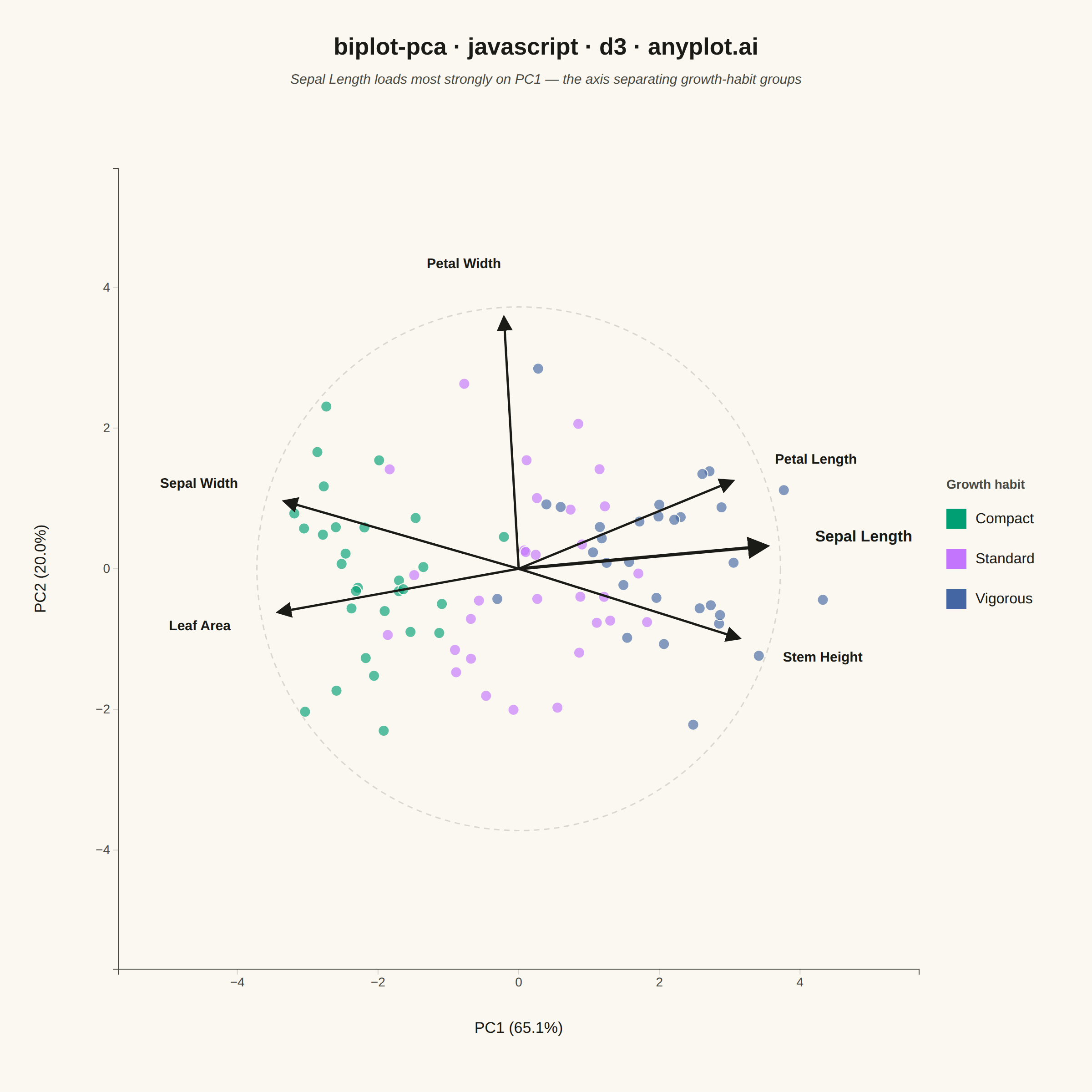
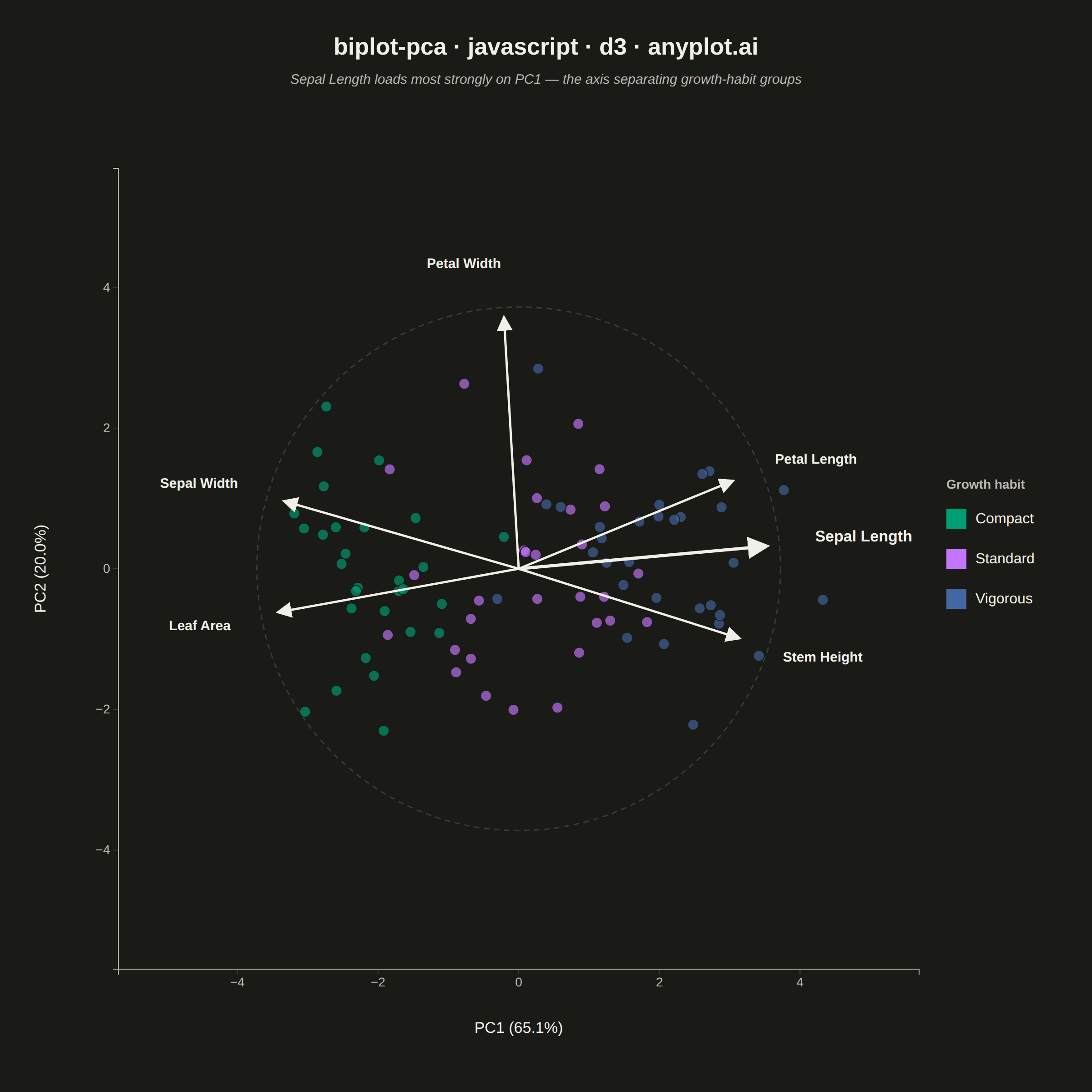
The same plot in 14 other libraries — JavaScript: Chart.js, Apache ECharts, Highcharts, MUI X Charts; Python: Altair, Bokeh, lets-plot, Matplotlib, Plotly, plotnine, Pygal, Seaborn; R: ggplot2; Julia: Makie.jl. Compare all 15 side by side: PCA Biplot with Scores and Loading Vectors in Python, R, Julia and JavaScript.
A PCA biplot simultaneously displays both observation scores (as points) and variable loadings (as arrows) in the principal component space. This dual representation is essential for interpreting PCA results, revealing how observations relate to each other and which original variables drive the separation along each principal component. The length and direction of loading arrows indicate variable importance and correlation with the components.
// anyplot.ai
// biplot-pca: PCA Biplot with Scores and Loading Vectors
// Library: d3 7.9.0 | JavaScript 22.23.2
// Quality: 90/100 | Created: 2026-09-01
//# anyplot-orientation: square

const t = window.ANYPLOT_TOKENS;
const { width, height } = window.ANYPLOT_SIZE;

// --- Data: synthetic plant morphology survey, 3 growth-habit groups -------
function lcg(seed) {
  let state = seed >>> 0;
  return () => {
    state = (state * 1664525 + 1013904223) >>> 0;
    return state / 4294967296;
  };
}
const rand = lcg(42);
function gaussian() {
  let u1 = 0;
  while (u1 === 0) u1 = rand();
  const u2 = rand();
  return Math.sqrt(-2 * Math.log(u1)) * Math.cos(2 * Math.PI * u2);
}

// Each feature loads on the two latent factors (size, shape) at its own angle,
// so the six loading arrows fan out around the circle instead of bunching up.
const featureSpecs = [
  { name: "Sepal Length", mean: 5.0, spread: 0.7, angleDeg: 10 },
  { name: "Petal Length", mean: 3.5, spread: 0.9, angleDeg: 55 },
  { name: "Petal Width", mean: 1.2, spread: 0.35, angleDeg: 95 },
  { name: "Sepal Width", mean: 3.0, spread: 0.4, angleDeg: 150 },
  { name: "Leaf Area", mean: 15, spread: 3.5, angleDeg: 205 },
  { name: "Stem Height", mean: 40, spread: 7, angleDeg: 320 },
];
const featureNames = featureSpecs.map((f) => f.name);
const groups = [
  { name: "Compact", sizeMean: -1.3 },
  { name: "Standard", sizeMean: 0 },
  { name: "Vigorous", sizeMean: 1.3 },
];

const observations = [];
for (const grp of groups) {
  for (let i = 0; i < 30; i++) {
    const size = grp.sizeMean + gaussian() * 0.5;
    const shape = gaussian() * 0.5;
    observations.push({
      group: grp.name,
      values: featureSpecs.map((f) => {
        const angleRad = (f.angleDeg * Math.PI) / 180;
        const signal = Math.cos(angleRad) * size + Math.sin(angleRad) * shape;
        return f.mean + f.spread * 0.9 * signal + gaussian() * f.spread * 0.45;
      }),
    });
  }
}

// --- Standardize columns, then PCA on the correlation matrix ---------------
const n = observations.length;
const p = featureNames.length;

const means = Array(p).fill(0);
for (const obs of observations) obs.values.forEach((v, j) => (means[j] += v / n));

const stds = Array(p).fill(0);
for (const obs of observations) obs.values.forEach((v, j) => (stds[j] += (v - means[j]) ** 2 / (n - 1)));
stds.forEach((s, j) => (stds[j] = Math.sqrt(s)));

const standardized = observations.map((obs) => obs.values.map((v, j) => (v - means[j]) / stds[j]));

const corr = Array.from({ length: p }, () => Array(p).fill(0));
for (let a = 0; a < p; a++) {
  for (let b = 0; b < p; b++) {
    let sum = 0;
    for (let i = 0; i < n; i++) sum += standardized[i][a] * standardized[i][b];
    corr[a][b] = sum / (n - 1);
  }
}

// Cyclic Jacobi eigenvalue algorithm for the symmetric correlation matrix
function jacobiEigen(matrix) {
  const dim = matrix.length;
  const a = matrix.map((row) => row.slice());
  const v = Array.from({ length: dim }, (_, i) => Array.from({ length: dim }, (_, j) => (i === j ? 1 : 0)));
  for (let sweep = 0; sweep < 100; sweep++) {
    let offDiag = 0;
    for (let i = 0; i < dim; i++) for (let j = i + 1; j < dim; j++) offDiag += a[i][j] * a[i][j];
    if (offDiag < 1e-12) break;
    for (let pi = 0; pi < dim; pi++) {
      for (let qi = pi + 1; qi < dim; qi++) {
        if (Math.abs(a[pi][qi]) < 1e-14) continue;
        const theta = (a[qi][qi] - a[pi][pi]) / (2 * a[pi][qi]);
        const tt = Math.sign(theta || 1) / (Math.abs(theta) + Math.sqrt(theta * theta + 1));
        const c = 1 / Math.sqrt(tt * tt + 1);
        const s = tt * c;
        const app = a[pi][pi];
        const aqq = a[qi][qi];
        const apq = a[pi][qi];
        a[pi][pi] = c * c * app - 2 * s * c * apq + s * s * aqq;
        a[qi][qi] = s * s * app + 2 * s * c * apq + c * c * aqq;
        a[pi][qi] = 0;
        a[qi][pi] = 0;
        for (let i = 0; i < dim; i++) {
          if (i === pi || i === qi) continue;
          const aip = a[i][pi];
          const aiq = a[i][qi];
          a[i][pi] = c * aip - s * aiq;
          a[pi][i] = a[i][pi];
          a[i][qi] = s * aip + c * aiq;
          a[qi][i] = a[i][qi];
        }
        for (let i = 0; i < dim; i++) {
          const vip = v[i][pi];
          const viq = v[i][qi];
          v[i][pi] = c * vip - s * viq;
          v[i][qi] = s * vip + c * viq;
        }
      }
    }
  }
  return { eigenvalues: Array.from({ length: dim }, (_, i) => a[i][i]), eigenvectors: v };
}

const { eigenvalues, eigenvectors } = jacobiEigen(corr);
const order = eigenvalues.map((_, idx) => idx).sort((a, b) => eigenvalues[b] - eigenvalues[a]);
const [pc1Idx, pc2Idx] = order;
const totalVariance = eigenvalues.reduce((sum, val) => sum + val, 0);
const pc1Pct = (eigenvalues[pc1Idx] / totalVariance) * 100;
const pc2Pct = (eigenvalues[pc2Idx] / totalVariance) * 100;

const scores = observations.map((obs, i) => {
  let pc1 = 0;
  let pc2 = 0;
  for (let j = 0; j < p; j++) {
    pc1 += standardized[i][j] * eigenvectors[j][pc1Idx];
    pc2 += standardized[i][j] * eigenvectors[j][pc2Idx];
  }
  return { group: obs.group, pc1, pc2 };
});

// Correlation-biplot loadings: variable-PC correlation, magnitude <= 1
const loadings = featureNames.map((name, j) => ({
  name,
  pc1: eigenvectors[j][pc1Idx] * Math.sqrt(eigenvalues[pc1Idx]),
  pc2: eigenvectors[j][pc2Idx] * Math.sqrt(eigenvalues[pc2Idx]),
}));

// The feature whose loading correlates most strongly with PC1 is the single
// best explanation for the group separation visible along that axis — call
// it out visually instead of leaving every arrow at the same default weight.
const topDriver = loadings.reduce((best, d) => (Math.abs(d.pc1) > Math.abs(best.pc1) ? d : best), loadings[0]);

const maxScoreRadius = d3.max(scores, (d) => Math.hypot(d.pc1, d.pc2));
const arrowScale = 0.85 * maxScoreRadius;
const extent = maxScoreRadius * 1.3;

// --- Layout: equal-aspect plot area so loading-vector angles read true -----
const margin = { top: 160, right: 190, bottom: 110, left: 130 };
const availW = width - margin.left - margin.right;
const availH = height - margin.top - margin.bottom;
const plotSize = Math.min(availW, availH);
const xOffset = margin.left + (availW - plotSize) / 2;
const yOffset = margin.top + (availH - plotSize) / 2;

const x = d3.scaleLinear().domain([-extent, extent]).range([xOffset, xOffset + plotSize]);
const y = d3.scaleLinear().domain([-extent, extent]).range([yOffset + plotSize, yOffset]);
const color = d3.scaleOrdinal().domain(groups.map((g) => g.name)).range(t.palette.slice(0, groups.length));

// --- SVG mount ---------------------------------------------------------------
const svg = d3.select("#container").append("svg").attr("width", width).attr("height", height);

svg
  .append("defs")
  .append("marker")
  .attr("id", "loading-arrowhead")
  .attr("viewBox", "0 0 10 10")
  .attr("refX", 8)
  .attr("refY", 5)
  .attr("markerWidth", 7)
  .attr("markerHeight", 7)
  .attr("orient", "auto-start-reverse")
  .append("path")
  .attr("d", "M 0 0 L 10 5 L 0 10 z")
  .attr("fill", t.ink);

// --- Unit circle: reference for correlation-loading magnitude --------------
svg
  .append("circle")
  .attr("cx", x(0))
  .attr("cy", y(0))
  .attr("r", x(arrowScale) - x(0))
  .attr("fill", "none")
  .attr("stroke", t.grid)
  .attr("stroke-width", 1.5)
  .attr("stroke-dasharray", "6,5");

// --- Axes ---------------------------------------------------------------------
const xAxisG = svg.append("g").attr("transform", `translate(0,${yOffset + plotSize})`).call(d3.axisBottom(x).ticks(6));
const yAxisG = svg.append("g").attr("transform", `translate(${xOffset},0)`).call(d3.axisLeft(y).ticks(6));
for (const axisG of [xAxisG, yAxisG]) {
  axisG.selectAll("text").attr("fill", t.inkSoft).style("font-size", "14px");
  axisG.selectAll("line").attr("stroke", t.grid);
  axisG.select(".domain").attr("stroke", t.inkSoft);
}

svg
  .append("text")
  .attr("x", xOffset + plotSize / 2)
  .attr("y", yOffset + plotSize + 70)
  .attr("text-anchor", "middle")
  .attr("fill", t.ink)
  .style("font-size", "17px")
  .text(`PC1 (${pc1Pct.toFixed(1)}%)`);

svg
  .append("text")
  .attr("transform", `translate(${xOffset - 80},${yOffset + plotSize / 2}) rotate(-90)`)
  .attr("text-anchor", "middle")
  .attr("fill", t.ink)
  .style("font-size", "17px")
  .text(`PC2 (${pc2Pct.toFixed(1)}%)`);

// --- Observation scores (drawn first so loading arrows/labels stay on top) -----
svg
  .selectAll(".score-point")
  .data(scores)
  .join("circle")
  .attr("cx", (d) => x(d.pc1))
  .attr("cy", (d) => y(d.pc2))
  .attr("r", 6)
  .attr("fill", (d) => color(d.group))
  .attr("fill-opacity", 0.65)
  .attr("stroke", t.pageBg)
  .attr("stroke-width", 1);

// --- Loading arrows + labels ---------------------------------------------------
svg
  .selectAll(".loading-arrow")
  .data(loadings)
  .join("line")
  .attr("x1", x(0))
  .attr("y1", y(0))
  .attr("x2", (d) => x(d.pc1 * arrowScale))
  .attr("y2", (d) => y(d.pc2 * arrowScale))
  .attr("stroke", t.ink)
  .attr("stroke-width", (d) => (d.name === topDriver.name ? 3.5 : 2.5))
  .attr("marker-end", "url(#loading-arrowhead)");

svg
  .selectAll(".loading-label")
  .data(loadings)
  .join("text")
  .attr("x", (d) => x(d.pc1 * arrowScale * 1.2))
  .attr("y", (d) => y(d.pc2 * arrowScale * 1.2))
  .attr("text-anchor", (d) => (d.pc1 >= 0 ? "start" : "end"))
  .attr("dominant-baseline", (d) => (d.pc2 >= 0 ? "auto" : "hanging"))
  .attr("fill", t.ink)
  .style("font-size", (d) => (d.name === topDriver.name ? "17px" : "15px"))
  .style("font-weight", (d) => (d.name === topDriver.name ? "700" : "600"))
  .style("paint-order", "stroke")
  .attr("stroke", t.pageBg)
  .attr("stroke-width", 6.5)
  .text((d) => d.name);

// --- Legend -----------------------------------------------------------------------
const legendX = xOffset + plotSize + 30;
const legendY = yOffset + plotSize / 2 - (groups.length * 44) / 2;
svg
  .append("text")
  .attr("x", legendX)
  .attr("y", legendY - 22)
  .attr("fill", t.inkSoft)
  .style("font-size", "14px")
  .style("font-weight", "600")
  .text("Growth habit");
groups.forEach((grp, i) => {
  const rowY = legendY + i * 44;
  svg.append("rect").attr("x", legendX).attr("y", rowY).attr("width", 22).attr("height", 22).attr("fill", color(grp.name));
  svg
    .append("text")
    .attr("x", legendX + 32)
    .attr("y", rowY + 16)
    .attr("fill", t.ink)
    .style("font-size", "16px")
    .text(grp.name);
});

// --- Title --------------------------------------------------------------------------
svg
  .append("text")
  .attr("x", width / 2)
  .attr("y", 60)
  .attr("text-anchor", "middle")
  .attr("fill", t.ink)
  .style("font-size", "26px")
  .style("font-weight", "600")
  .text("biplot-pca · javascript · d3 · anyplot.ai");

// Subtitle: call out the strongest driver of the PC1 separation seen in the
// scores below, so the story is more than "points happen to cluster by color".
svg
  .append("text")
  .attr("x", width / 2)
  .attr("y", 92)
  .attr("text-anchor", "middle")
  .attr("fill", t.inkSoft)
  .style("font-size", "15px")
  .style("font-style", "italic")
  .text(`${topDriver.name} loads most strongly on PC1 — the axis separating growth-habit groups`);
Runnable source as JSON, for any HTTP client: https://api.anyplot.ai/specs/biplot-pca/d3/code. Any spec id and library id listed in llms-full.txt fit the same URL shape; every URL below is complete and callable.
{
  "spec_id": "biplot-pca",
  "language": "javascript",
  "library": "d3",
  "page": "https://anyplot.ai/biplot-pca/javascript/d3",
  "hub": "https://anyplot.ai/biplot-pca",
  "code_json": "https://api.anyplot.ai/specs/biplot-pca/d3/code",
  "spec_json": "https://api.anyplot.ai/specs/biplot-pca",
  "render_light_png": "https://storage.googleapis.com/anyplot-images/plots/biplot-pca/javascript/d3/plot-light.png",
  "render_dark_png": "https://storage.googleapis.com/anyplot-images/plots/biplot-pca/javascript/d3/plot-dark.png",
  "interactive_light_html": "https://storage.googleapis.com/anyplot-images/plots/biplot-pca/javascript/d3/plot-light.html",
  "interactive_dark_html": "https://storage.googleapis.com/anyplot-images/plots/biplot-pca/javascript/d3/plot-dark.html",
  "quality_score": 90.0,
  "license": "MIT",
  "guide": "https://anyplot.ai/llms.txt"
}
Part of PCA Biplot with Scores and Loading Vectors on anyplot.ai.