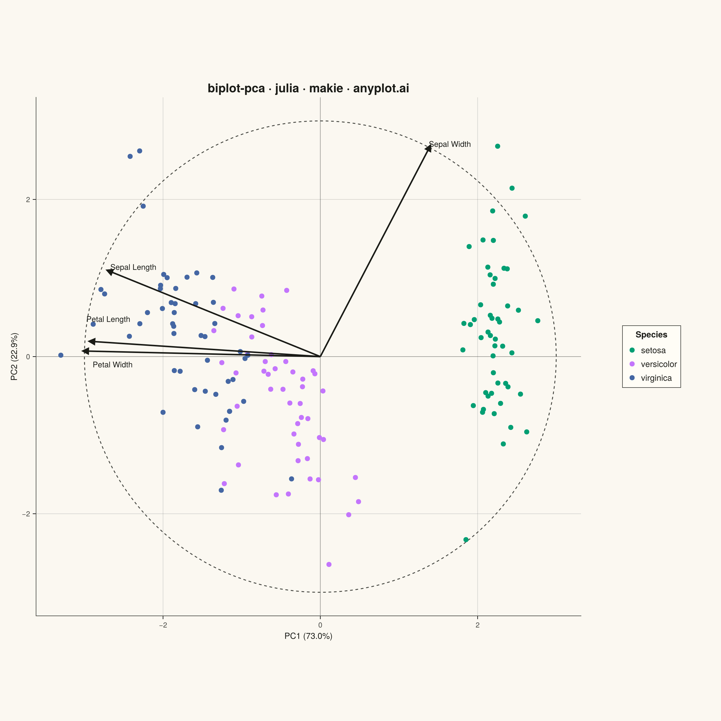
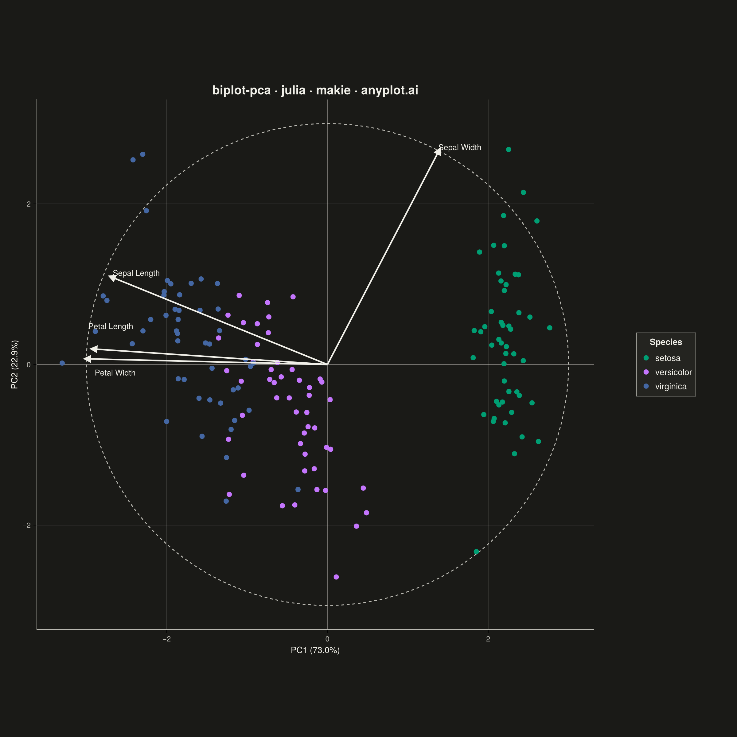
The same plot in 14 other libraries — Python: Altair, Bokeh, lets-plot, Matplotlib, Plotly, plotnine, Pygal, Seaborn; R: ggplot2; JavaScript: Chart.js, D3.js, Apache ECharts, Highcharts, MUI X Charts. Compare all 15 side by side: PCA Biplot with Scores and Loading Vectors in Python, R, Julia and JavaScript.
A PCA biplot simultaneously displays both observation scores (as points) and variable loadings (as arrows) in the principal component space. This dual representation is essential for interpreting PCA results, revealing how observations relate to each other and which original variables drive the separation along each principal component. The length and direction of loading arrows indicate variable importance and correlation with the components.
# anyplot.ai
# biplot-pca: PCA Biplot with Scores and Loading Vectors
# Library: makie 0.21.9 | Julia 1.11.9
# Quality: 88/100 | Created: 2026-09-01

using CairoMakie
using Colors
using RDatasets
using Statistics
using LinearAlgebra

# --- Theme tokens ------------------------------------------------------------
const THEME       = get(ENV, "ANYPLOT_THEME", "light")
const PAGE_BG     = THEME == "light" ? colorant"#FAF8F1" : colorant"#1A1A17"
const INK         = THEME == "light" ? colorant"#1A1A17" : colorant"#F0EFE8"
const INK_SOFT    = THEME == "light" ? colorant"#4A4A44" : colorant"#B8B7B0"
const IMPRINT_PALETTE = [
    colorant"#009E73", colorant"#C475FD", colorant"#4467A3", colorant"#BD8233",
    colorant"#AE3030", colorant"#2ABCCD", colorant"#954477", colorant"#99B314",
]

# --- Data ---------------------------------------------------------------------
iris = RDatasets.dataset("datasets", "iris")
feature_names = ["Sepal Length", "Sepal Width", "Petal Length", "Petal Width"]
features = Matrix(iris[:, [:SepalLength, :SepalWidth, :PetalLength, :PetalWidth]])
species = String.(iris.Species)
groups = unique(species)

# Standardize so PCA decomposes the correlation matrix, not the covariance matrix
feature_means = mean(features; dims = 1)
feature_stds = std(features; dims = 1)
standardized = (features .- feature_means) ./ feature_stds

# Eigen-decompose the correlation matrix, sorted by descending eigenvalue
correlation = Symmetric(cor(standardized))
eigen_result = eigen(correlation)
order = sortperm(eigen_result.values; rev = true)
eigenvalues = eigen_result.values[order]
eigenvectors = eigen_result.vectors[:, order]

variance_explained = eigenvalues ./ sum(eigenvalues) .* 100
scores = standardized * eigenvectors[:, 1:2]
loadings = eigenvectors[:, 1:2] .* sqrt.(eigenvalues[1:2])'

# Scale correlation loadings so the arrows sit alongside the score cloud
score_radius = maximum(sqrt.(scores[:, 1] .^ 2 .+ scores[:, 2] .^ 2))
loading_radius = maximum(sqrt.(loadings[:, 1] .^ 2 .+ loadings[:, 2] .^ 2))
arrow_scale = 0.85 * score_radius / loading_radius
arrow_xy = loadings .* arrow_scale

# --- Plot -----------------------------------------------------------------
fig = Figure(
    resolution      = (1200, 1200),
    fontsize        = 14,
    backgroundcolor = PAGE_BG,
    figure_padding  = (10, 10, 10, 10),
)

pc1_label = "PC1 ($(round(variance_explained[1]; digits = 1))%)"
pc2_label = "PC2 ($(round(variance_explained[2]; digits = 1))%)"

ax = Axis(
    fig[1, 1];
    title              = "biplot-pca · julia · makie · anyplot.ai",
    titlesize          = 20,
    titlecolor         = INK,
    xlabel             = pc1_label,
    ylabel             = pc2_label,
    xlabelcolor        = INK,
    ylabelcolor        = INK,
    xlabelsize         = 14,
    ylabelsize         = 14,
    xticklabelcolor    = INK_SOFT,
    yticklabelcolor    = INK_SOFT,
    xticklabelsize     = 12,
    yticklabelsize     = 12,
    backgroundcolor    = PAGE_BG,
    topspinevisible    = false,
    rightspinevisible  = false,
    leftspinecolor     = INK_SOFT,
    bottomspinecolor   = INK_SOFT,
    xgridcolor         = RGBAf(INK.r, INK.g, INK.b, 0.15),
    ygridcolor         = RGBAf(INK.r, INK.g, INK.b, 0.15),
    xautolimitmargin   = (0.03, 0.03),
    yautolimitmargin   = (0.03, 0.03),
    aspect             = DataAspect(),
)

# Unit circle reference for the correlation-scaled loadings
circle_theta = range(0, 2π; length = 200)
lines!(ax, cos.(circle_theta) .* arrow_scale, sin.(circle_theta) .* arrow_scale;
    color = INK_SOFT, linestyle = :dash, linewidth = 1.5)

hlines!(ax, [0]; color = RGBAf(INK.r, INK.g, INK.b, 0.3), linewidth = 1)
vlines!(ax, [0]; color = RGBAf(INK.r, INK.g, INK.b, 0.3), linewidth = 1)

# Subtle per-group 1.5σ density ellipses give the species separation a
# deliberate focal point instead of relying on point color alone
ellipse_theta = range(0, 2π; length = 100)
for (i, group) in enumerate(groups)
    mask = species .== group
    group_scores = scores[mask, :]
    center = vec(mean(group_scores; dims = 1))
    group_evals, group_evecs = eigen(Symmetric(cov(group_scores)))
    group_order = sortperm(group_evals; rev = true)
    radii = 1.5 .* sqrt.(max.(group_evals[group_order], 0))
    circle_pts = radii .* permutedims(hcat(cos.(ellipse_theta), sin.(ellipse_theta)))
    ellipse_pts = group_evecs[:, group_order] * circle_pts
    poly!(ax, Point2f.(ellipse_pts[1, :] .+ center[1], ellipse_pts[2, :] .+ center[2]);
        color = (IMPRINT_PALETTE[i], 0.10), strokecolor = (IMPRINT_PALETTE[i], 0.35), strokewidth = 1)
end

for (i, group) in enumerate(groups)
    mask = species .== group
    scatter!(ax, scores[mask, 1], scores[mask, 2];
        color = IMPRINT_PALETTE[i], markersize = 12, strokewidth = 0, label = group)
end

# Heavier line weight for the dominant loadings makes the strongest drivers
# of variance the clear focal point rather than four uniform arrows
loading_magnitude = sqrt.(arrow_xy[:, 1] .^ 2 .+ arrow_xy[:, 2] .^ 2)
arrow_linewidth = 1.8 .+ 1.8 .* (loading_magnitude ./ maximum(loading_magnitude))

arrows!(ax, zeros(length(feature_names)), zeros(length(feature_names)),
    arrow_xy[:, 1], arrow_xy[:, 2];
    color = INK, linewidth = arrow_linewidth, arrowsize = 18)

# Nudge labels apart vertically when their arrow tips sit too close to read
label_offset = zeros(length(feature_names), 2)
for i in 1:length(feature_names), j in (i + 1):length(feature_names)
    tip_distance = hypot(arrow_xy[i, 1] - arrow_xy[j, 1], arrow_xy[i, 2] - arrow_xy[j, 2])
    if tip_distance < 0.4
        label_offset[i, 2] += 0.35
        label_offset[j, 2] -= 0.35
    end
end

# Anchor each label on whichever horizontal side has more clearance from the
# score cloud, so the text itself never runs into a nearby point cluster
# (a fixed left-anchor would run "Sepal Width" straight into the setosa
# points sitting just beyond its arrow tip)
text_halfwidth = [0.025 * length(name) for name in feature_names]
h_align = Vector{Symbol}(undef, length(feature_names))
for i in 1:length(feature_names)
    tip = arrow_xy[i, :] .+ label_offset[i, :]
    right_center = tip .+ [text_halfwidth[i], 0]
    left_center = tip .- [text_halfwidth[i], 0]
    dist_right = minimum(hypot.(scores[:, 1] .- right_center[1], scores[:, 2] .- right_center[2]))
    dist_left = minimum(hypot.(scores[:, 1] .- left_center[1], scores[:, 2] .- left_center[2]))
    h_align[i] = dist_right >= dist_left ? :left : :right
end

for (i, name) in enumerate(feature_names)
    text!(ax, arrow_xy[i, 1] + label_offset[i, 1], arrow_xy[i, 2] + label_offset[i, 2]; text = name,
        color = INK, fontsize = 13, align = (h_align[i], :bottom))
end

Legend(fig[1, 2], ax, "Species";
    framevisible = false, labelcolor = INK, titlecolor = INK)
colsize!(fig.layout, 2, Relative(0.15))
colgap!(fig.layout, 1, 8)

# --- Save -------------------------------------------------------------------
save("plot-$(THEME).png", fig; px_per_unit = 2)
Runnable source as JSON, for any HTTP client: https://api.anyplot.ai/specs/biplot-pca/makie/code. Any spec id and library id listed in llms-full.txt fit the same URL shape; every URL below is complete and callable.
{
  "spec_id": "biplot-pca",
  "language": "julia",
  "library": "makie",
  "page": "https://anyplot.ai/biplot-pca/julia/makie",
  "hub": "https://anyplot.ai/biplot-pca",
  "code_json": "https://api.anyplot.ai/specs/biplot-pca/makie/code",
  "spec_json": "https://api.anyplot.ai/specs/biplot-pca",
  "render_light_png": "https://storage.googleapis.com/anyplot-images/plots/biplot-pca/julia/makie/plot-light.png",
  "render_dark_png": "https://storage.googleapis.com/anyplot-images/plots/biplot-pca/julia/makie/plot-dark.png",
  "quality_score": 88.0,
  "license": "MIT",
  "guide": "https://anyplot.ai/llms.txt"
}
Part of PCA Biplot with Scores and Loading Vectors on anyplot.ai.