The same plot in 14 other libraries — Python: Bokeh, lets-plot, Matplotlib, Plotly, plotnine, Pygal, Seaborn; R: ggplot2; Julia: Makie.jl; JavaScript: Chart.js, D3.js, Apache ECharts, Highcharts, MUI X Charts. Compare all 15 side by side: Route Path Map in Python, R, Julia and JavaScript.
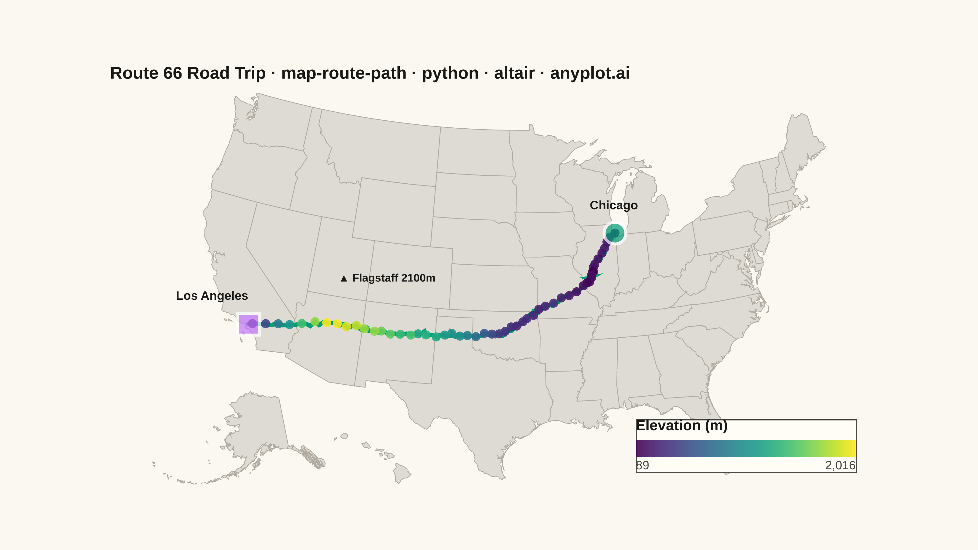
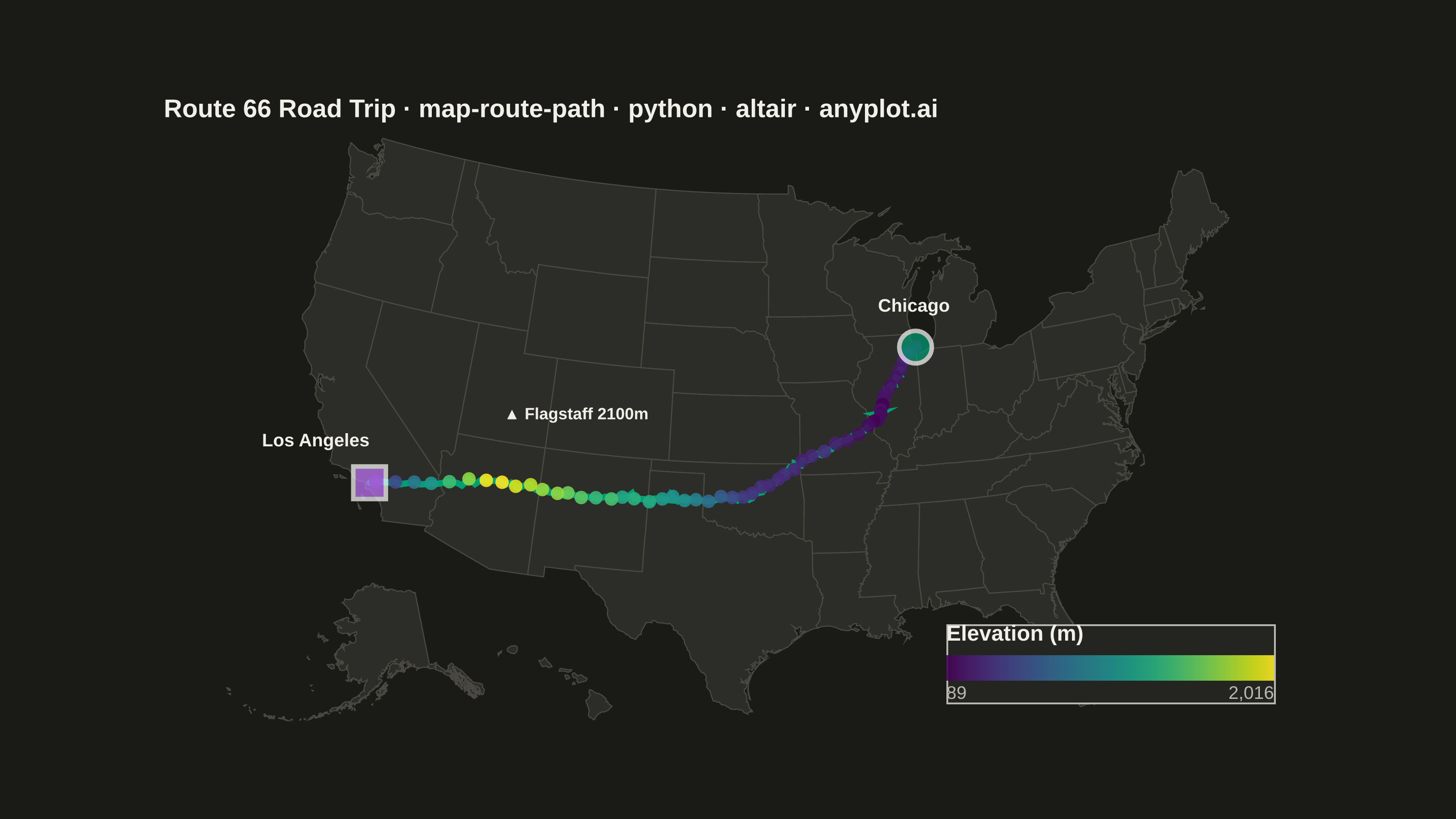
A geographic map visualization showing a connected path or route between sequential waypoints. Unlike scatter maps that display discrete points, this plot connects coordinates in order to reveal journeys, tracks, and navigation paths. Ideal for GPS data, delivery routes, and travel visualization where the sequence and continuity of movement matters.
""" anyplot.ai
map-route-path: Route Path Map
Library: altair 6.1.0 | Python 3.13.13
Quality: 91/100 | Created: 2026-05-21
"""

import os
import sys


sys.path.pop(0)  # prevent local altair.py from shadowing the library
import altair as alt
import numpy as np
import pandas as pd
from PIL import Image


# Theme tokens
THEME = os.getenv("ANYPLOT_THEME", "light")
PAGE_BG = "#FAF8F1" if THEME == "light" else "#1A1A17"
ELEVATED_BG = "#FFFDF6" if THEME == "light" else "#242420"
INK = "#1A1A17" if THEME == "light" else "#F0EFE8"
INK_SOFT = "#4A4A44" if THEME == "light" else "#B8B7B0"
MAP_FILL = "#DEDAD4" if THEME == "light" else "#2C2C28"
MAP_STROKE = "#B0AAA0" if THEME == "light" else "#4A4A42"

# Data — Route 66: Chicago → Los Angeles (8 segments, ~160 synthetic waypoints)
np.random.seed(42)

city_coords = [
    (41.85, -87.65),  # Chicago, IL
    (39.80, -89.65),  # Springfield, IL
    (38.63, -90.20),  # St. Louis, MO
    (37.08, -94.52),  # Joplin, MO
    (35.47, -97.52),  # Oklahoma City, OK
    (35.22, -101.83),  # Amarillo, TX
    (35.08, -106.65),  # Albuquerque, NM
    (35.20, -111.65),  # Flagstaff, AZ
    (34.05, -118.25),  # Los Angeles, CA
]
city_elevations = [180, 165, 130, 290, 365, 1100, 1510, 2100, 95]

rows = []
seq = 0
for i in range(len(city_coords) - 1):
    lat1, lon1 = city_coords[i]
    lat2, lon2 = city_coords[i + 1]
    n = 20
    t_vals = np.linspace(0, 1, n + 1)[:-1]
    lats = lat1 + (lat2 - lat1) * t_vals + np.random.normal(0, 0.07, n)
    lons = lon1 + (lon2 - lon1) * t_vals + np.random.normal(0, 0.07, n)
    for j in range(n):
        rows.append({"lat": lats[j], "lon": lons[j], "sequence": seq})
        seq += 1
rows.append({"lat": city_coords[-1][0], "lon": city_coords[-1][1], "sequence": seq})
df = pd.DataFrame(rows)

city_s = np.linspace(0, 1, len(city_coords))
route_s = df["sequence"].values / df["sequence"].max()
df["elevation_m"] = np.interp(route_s, city_s, city_elevations) + np.random.normal(0, 45, len(df))

start_df = df.iloc[[0]].copy()
start_df["label"] = "Start: Chicago, IL"
end_df = df.iloc[[-1]].copy()
end_df["label"] = "End: Los Angeles, CA"
dot_df = df.iloc[::3].reset_index(drop=True)

# City label DataFrames (separate layers needed for different per-label alignment)
chicago_ldf = pd.DataFrame([{"lon": city_coords[0][1], "lat": city_coords[0][0], "label": "Chicago"}])
la_ldf = pd.DataFrame([{"lon": city_coords[-1][1], "lat": city_coords[-1][0], "label": "Los Angeles"}])
flagstaff_ldf = pd.DataFrame([{"lon": city_coords[7][1], "lat": city_coords[7][0], "label": "▲ Flagstaff 2100m"}])

title_str = "Route 66 Road Trip · map-route-path · python · altair · anyplot.ai"

# Basemap: US states (CDN topojson, no local package required)
us_url = "https://cdn.jsdelivr.net/npm/vega-datasets@2/data/us-10m.json"
states = alt.topo_feature(us_url, "states")

# Map layers
background = (
    alt.Chart(states)
    .mark_geoshape(fill=MAP_FILL, stroke=MAP_STROKE, strokeWidth=0.6)
    .project(type="albersUsa")
    .properties(width=620, height=320)
)

route_line = (
    alt.Chart(df)
    .mark_line(strokeWidth=3.5, color="#009E73", strokeCap="round")
    .encode(
        longitude="lon:Q",
        latitude="lat:Q",
        order="sequence:O",
        tooltip=[
            alt.Tooltip("lat:Q", title="Latitude", format=".2f"),
            alt.Tooltip("lon:Q", title="Longitude", format=".2f"),
            alt.Tooltip("elevation_m:Q", title="Elevation (m)", format=".0f"),
        ],
    )
    .project(type="albersUsa")
)

elevation_dots = (
    alt.Chart(dot_df)
    .mark_circle(size=55, opacity=0.9)
    .encode(
        longitude="lon:Q",
        latitude="lat:Q",
        color=alt.Color(
            "elevation_m:Q",
            scale=alt.Scale(scheme="viridis"),
            legend=alt.Legend(
                title="Elevation (m)",
                titleFontSize=12,
                labelFontSize=10,
                gradientLength=180,
                gradientThickness=14,
                orient="bottom-right",
                offset=10,
            ),
        ),
        order="sequence:O",
        tooltip=[alt.Tooltip("elevation_m:Q", title="Elevation (m)", format=".0f")],
    )
    .project(type="albersUsa")
)

start_marker = (
    alt.Chart(start_df)
    .mark_point(shape="circle", size=320, filled=True, color="#009E73", stroke="white", strokeWidth=2.5)
    .encode(longitude="lon:Q", latitude="lat:Q", tooltip="label:N")
    .project(type="albersUsa")
)

end_marker = (
    alt.Chart(end_df)
    .mark_point(shape="square", size=320, filled=True, color="#C475FD", stroke="white", strokeWidth=2.5)
    .encode(longitude="lon:Q", latitude="lat:Q", tooltip="label:N")
    .project(type="albersUsa")
)

# Chicago: center-aligned above the start marker
chicago_label = (
    alt.Chart(chicago_ldf)
    .mark_text(fontSize=10, fontWeight="bold", dy=-18, baseline="bottom", align="center")
    .encode(longitude="lon:Q", latitude="lat:Q", text="label:N", color=alt.value(INK))
    .project(type="albersUsa")
)

# Los Angeles: right-aligned (text extends west, clear of Flagstaff overlap)
la_label = (
    alt.Chart(la_ldf)
    .mark_text(fontSize=10, fontWeight="bold", dy=-18, baseline="bottom", align="right")
    .encode(longitude="lon:Q", latitude="lat:Q", text="label:N", color=alt.value(INK))
    .project(type="albersUsa")
)

# Flagstaff elevation peak: left-aligned + higher offset, extends east away from LA label
flagstaff_label = (
    alt.Chart(flagstaff_ldf)
    .mark_text(fontSize=9, fontWeight="bold", dy=-32, baseline="bottom", align="left", dx=6)
    .encode(longitude="lon:Q", latitude="lat:Q", text="label:N", color=alt.value(INK))
    .project(type="albersUsa")
)

chart = (
    (background + route_line + elevation_dots + start_marker + end_marker + chicago_label + la_label + flagstaff_label)
    .properties(background=PAGE_BG, title=alt.Title(text=title_str, fontSize=14, anchor="start", color=INK, offset=8))
    .configure_view(fill=PAGE_BG, strokeWidth=0)
    .configure_title(color=INK)
    .configure_legend(fillColor=ELEVATED_BG, strokeColor=INK_SOFT, labelColor=INK_SOFT, titleColor=INK)
)

# Save PNG + HTML
TW, TH = 3200, 1800
chart.save(f"plot-{THEME}.png", scale_factor=4.0)
chart.save(f"plot-{THEME}.html")

# Canvas check: pad to target, raise on overshoot
_img = Image.open(f"plot-{THEME}.png").convert("RGB")
_w, _h = _img.size
if _w > TW or _h > TH:
    raise SystemExit(
        f"altair vl-convert produced {_w}×{_h}, exceeds target {TW}×{TH}. "
        f"Shrink chart .properties(width=, height=) values and re-render."
    )
if _w < TW or _h < TH:
    _canvas = Image.new("RGB", (TW, TH), PAGE_BG)
    _canvas.paste(_img, ((TW - _w) // 2, (TH - _h) // 2))
    _canvas.save(f"plot-{THEME}.png")
Runnable source as JSON, for any HTTP client: https://api.anyplot.ai/specs/map-route-path/altair/code. Any spec id and library id listed in llms-full.txt fit the same URL shape; every URL below is complete and callable.
{
  "spec_id": "map-route-path",
  "language": "python",
  "library": "altair",
  "page": "https://anyplot.ai/map-route-path/python/altair",
  "hub": "https://anyplot.ai/map-route-path",
  "code_json": "https://api.anyplot.ai/specs/map-route-path/altair/code",
  "spec_json": "https://api.anyplot.ai/specs/map-route-path",
  "render_light_png": "https://storage.googleapis.com/anyplot-images/plots/map-route-path/python/altair/plot-light.png",
  "render_dark_png": "https://storage.googleapis.com/anyplot-images/plots/map-route-path/python/altair/plot-dark.png",
  "interactive_light_html": "https://storage.googleapis.com/anyplot-images/plots/map-route-path/python/altair/plot-light.html",
  "interactive_dark_html": "https://storage.googleapis.com/anyplot-images/plots/map-route-path/python/altair/plot-dark.html",
  "quality_score": 91.0,
  "license": "MIT",
  "guide": "https://anyplot.ai/llms.txt"
}
Part of Route Path Map on anyplot.ai.