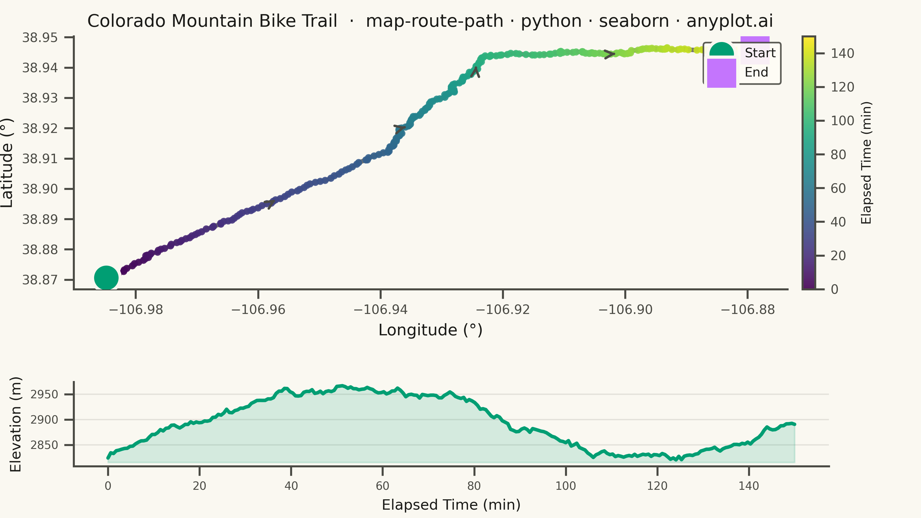
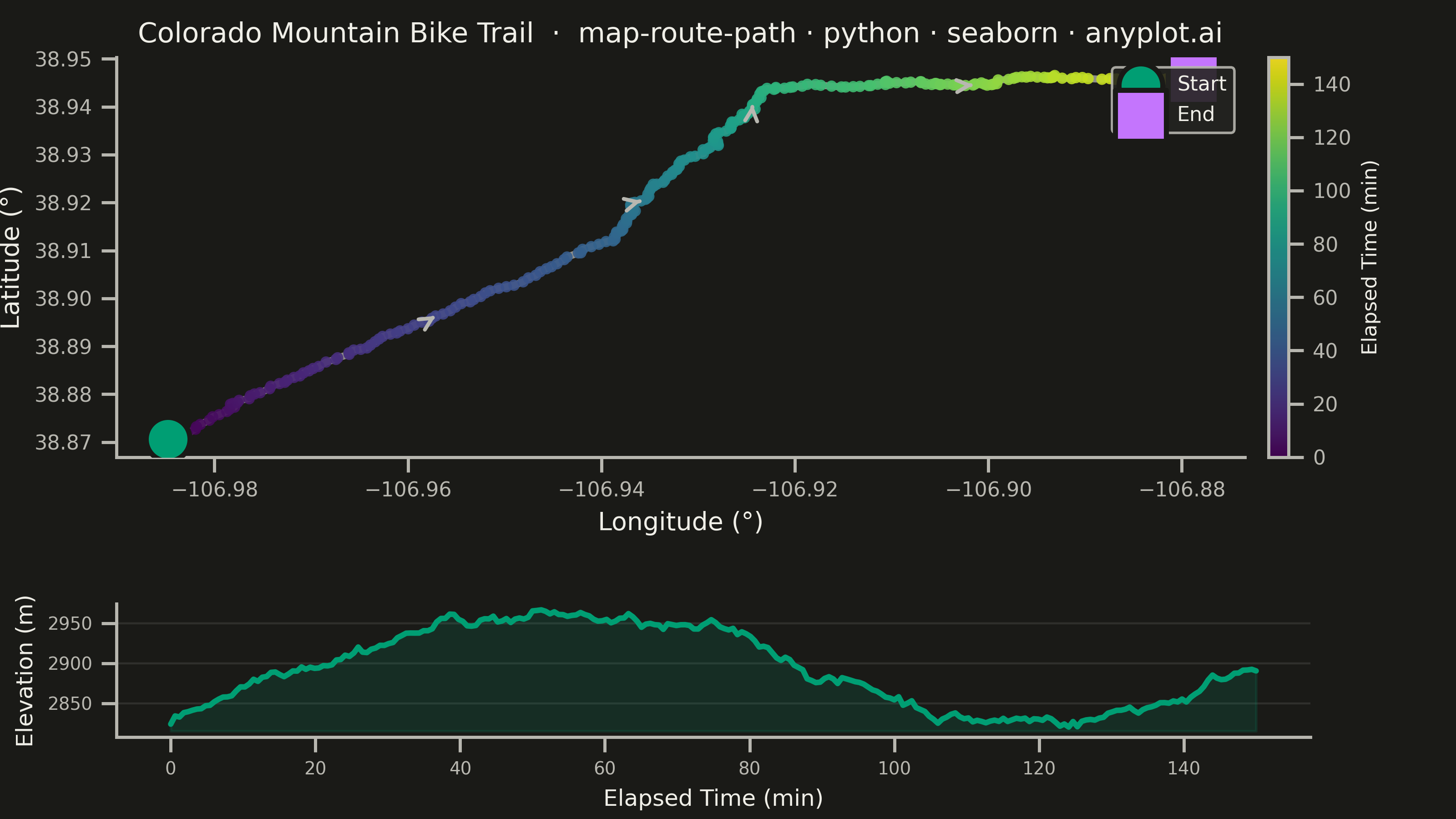
A geographic map visualization showing a connected path or route between sequential waypoints. Unlike scatter maps that display discrete points, this plot connects coordinates in order to reveal journeys, tracks, and navigation paths. Ideal for GPS data, delivery routes, and travel visualization where the sequence and continuity of movement matters.
""" anyplot.ai
map-route-path: Route Path Map
Library: seaborn 0.13.2 | Python 3.13.13
Quality: 87/100 | Updated: 2026-05-21
"""

import os

import matplotlib.pyplot as plt
import numpy as np
import pandas as pd
import seaborn as sns


# Theme tokens
THEME = os.getenv("ANYPLOT_THEME", "light")
PAGE_BG = "#FAF8F1" if THEME == "light" else "#1A1A17"
ELEVATED_BG = "#FFFDF6" if THEME == "light" else "#242420"
INK = "#1A1A17" if THEME == "light" else "#F0EFE8"
INK_SOFT = "#4A4A44" if THEME == "light" else "#B8B7B0"
BRAND = "#009E73"  # Okabe-Ito position 1 — always first series

sns.set_theme(
    style="ticks",
    rc={
        "figure.facecolor": PAGE_BG,
        "axes.facecolor": PAGE_BG,
        "axes.edgecolor": INK_SOFT,
        "axes.labelcolor": INK,
        "text.color": INK,
        "xtick.color": INK_SOFT,
        "ytick.color": INK_SOFT,
        "grid.color": INK,
        "grid.alpha": 0.10,
        "legend.facecolor": ELEVATED_BG,
        "legend.edgecolor": INK_SOFT,
    },
)

# Data — mountain bike trail GPS track near Crested Butte, Colorado
np.random.seed(42)
n_points = 250

start_lat, start_lon = 38.870, -106.985

lat_steps = np.random.normal(0.0003, 0.0002, n_points)
lon_steps = np.random.normal(0.0004, 0.0003, n_points)
lat_steps[:80] += 0.00025
lon_steps[:80] += 0.00015
lat_steps[80:160] += 0.00010
lon_steps[80:160] -= 0.00020
lat_steps[160:] -= 0.00030
lon_steps[160:] += 0.00010

lats = start_lat + np.cumsum(lat_steps)
lons = start_lon + np.cumsum(lon_steps)

base_elev = 2820
elevation = (
    base_elev + np.cumsum(np.random.normal(0.8, 3.5, n_points)) + 120 * np.sin(np.linspace(0, 1.8 * np.pi, n_points))
)

elapsed_min = np.linspace(0, 150, n_points)

df = pd.DataFrame({"lat": lats, "lon": lons, "elapsed_min": elapsed_min, "elevation_m": elevation})

# Figure: route map (top) + elevation profile (bottom)
fig, (ax_map, ax_elev) = plt.subplots(
    2, 1, figsize=(8, 4.5), dpi=400, gridspec_kw={"height_ratios": [3, 1]}, facecolor=PAGE_BG
)
fig.subplots_adjust(left=0.08, right=0.90, top=0.93, bottom=0.10, hspace=0.55)
ax_map.set_facecolor(PAGE_BG)
ax_elev.set_facecolor(PAGE_BG)

# Connecting path — strong line for clear route continuity
sns.lineplot(data=df, x="lon", y="lat", color=INK_SOFT, linewidth=2.8, alpha=0.75, ax=ax_map, sort=False, zorder=1)

# Waypoints colored by elapsed time (viridis — perceptually uniform sequential)
sc = ax_map.scatter(
    df["lon"], df["lat"], c=df["elapsed_min"], cmap="viridis", s=20, alpha=0.9, zorder=2, edgecolors="none"
)

# Start — Okabe-Ito position 1 (brand green)
ax_map.scatter(
    df["lon"].iloc[0],
    df["lat"].iloc[0],
    c=BRAND,
    s=300,
    marker="o",
    edgecolors=PAGE_BG,
    linewidths=2,
    zorder=5,
    label="Start",
)

# End — Okabe-Ito position 2 (vermillion) — larger to distinguish from dense viridis cluster
ax_map.scatter(
    df["lon"].iloc[-1],
    df["lat"].iloc[-1],
    c="#C475FD",
    s=400,
    marker="s",
    edgecolors=PAGE_BG,
    linewidths=2,
    zorder=5,
    label="End",
)

# Direction arrows along the path
for idx in [50, 100, 150, 200]:
    ax_map.annotate(
        "",
        xy=(df["lon"].iloc[idx + 1], df["lat"].iloc[idx + 1]),
        xytext=(df["lon"].iloc[idx], df["lat"].iloc[idx]),
        arrowprops={"arrowstyle": "->", "color": INK_SOFT, "lw": 1.5},
        zorder=3,
    )

# Colorbar for elapsed time
cbar = plt.colorbar(sc, ax=ax_map, pad=0.02, fraction=0.035)
cbar.set_label("Elapsed Time (min)", fontsize=8, color=INK)
cbar.ax.tick_params(labelsize=8, colors=INK_SOFT)
cbar.outline.set_edgecolor(INK_SOFT)

ax_map.set_xlabel("Longitude (°)", fontsize=10, color=INK)
ax_map.set_ylabel("Latitude (°)", fontsize=10, color=INK)
ax_map.set_title(
    "Colorado Mountain Bike Trail  ·  map-route-path · python · seaborn · anyplot.ai",
    fontsize=11,
    fontweight="medium",
    color=INK,
)
ax_map.tick_params(axis="both", labelsize=8)
ax_map.legend(fontsize=8, loc="upper right", framealpha=0.9)
sns.despine(ax=ax_map)

# Elevation profile — seaborn lineplot with fill for area under curve
sns.lineplot(data=df, x="elapsed_min", y="elevation_m", color=BRAND, linewidth=2.2, ax=ax_elev)
ax_elev.fill_between(df["elapsed_min"], df["elevation_m"].min() - 5, df["elevation_m"], alpha=0.15, color=BRAND)

ax_elev.set_xlabel("Elapsed Time (min)", fontsize=9, color=INK)
ax_elev.set_ylabel("Elevation (m)", fontsize=9, color=INK)
ax_elev.tick_params(axis="both", labelsize=7)
ax_elev.yaxis.grid(True, alpha=0.10, linewidth=0.8)
sns.despine(ax=ax_elev)

plt.savefig(f"plot-{THEME}.png", dpi=400, facecolor=PAGE_BG)
Runnable source as JSON, for any HTTP client: https://api.anyplot.ai/specs/map-route-path/seaborn/code. Any spec id and library id listed in llms-full.txt fit the same URL shape; every URL below is complete and callable.
{
  "spec_id": "map-route-path",
  "language": "python",
  "library": "seaborn",
  "page": "https://anyplot.ai/map-route-path/python/seaborn",
  "hub": "https://anyplot.ai/map-route-path",
  "code_json": "https://api.anyplot.ai/specs/map-route-path/seaborn/code",
  "spec_json": "https://api.anyplot.ai/specs/map-route-path",
  "render_light_png": "https://storage.googleapis.com/anyplot-images/plots/map-route-path/python/seaborn/plot-light.png",
  "render_dark_png": "https://storage.googleapis.com/anyplot-images/plots/map-route-path/python/seaborn/plot-dark.png",
  "quality_score": 87.0,
  "license": "MIT",
  "guide": "https://anyplot.ai/llms.txt"
}
Part of Route Path Map on anyplot.ai.