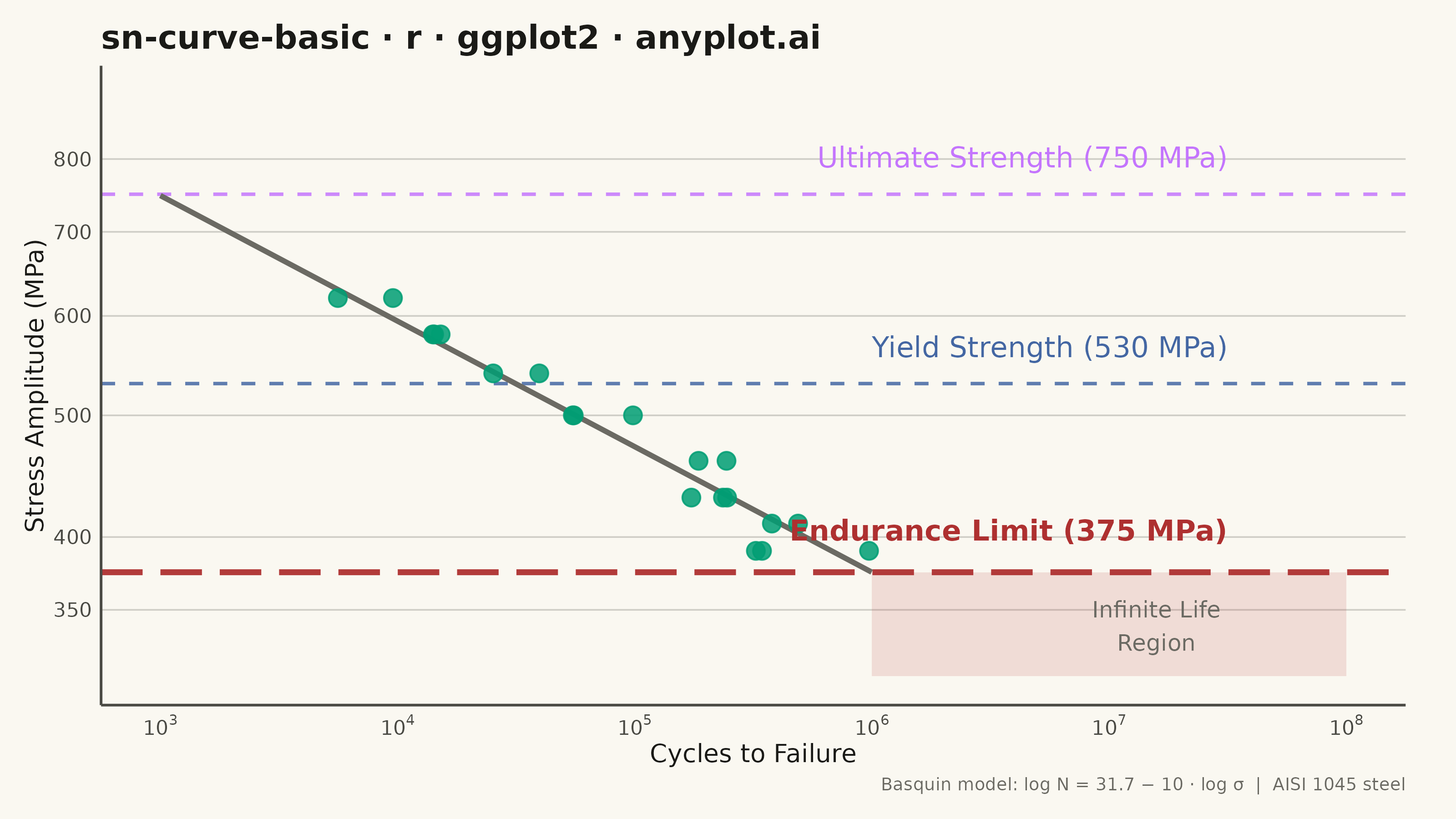
The same plot in 14 other libraries — Python: Altair, Bokeh, lets-plot, Matplotlib, Plotly, plotnine, Pygal, Seaborn; Julia: Makie.jl; JavaScript: Chart.js, D3.js, Apache ECharts, Highcharts, MUI X Charts. Compare all 15 side by side: S-N Curve (Wöhler Curve) in Python, R, Julia and JavaScript.
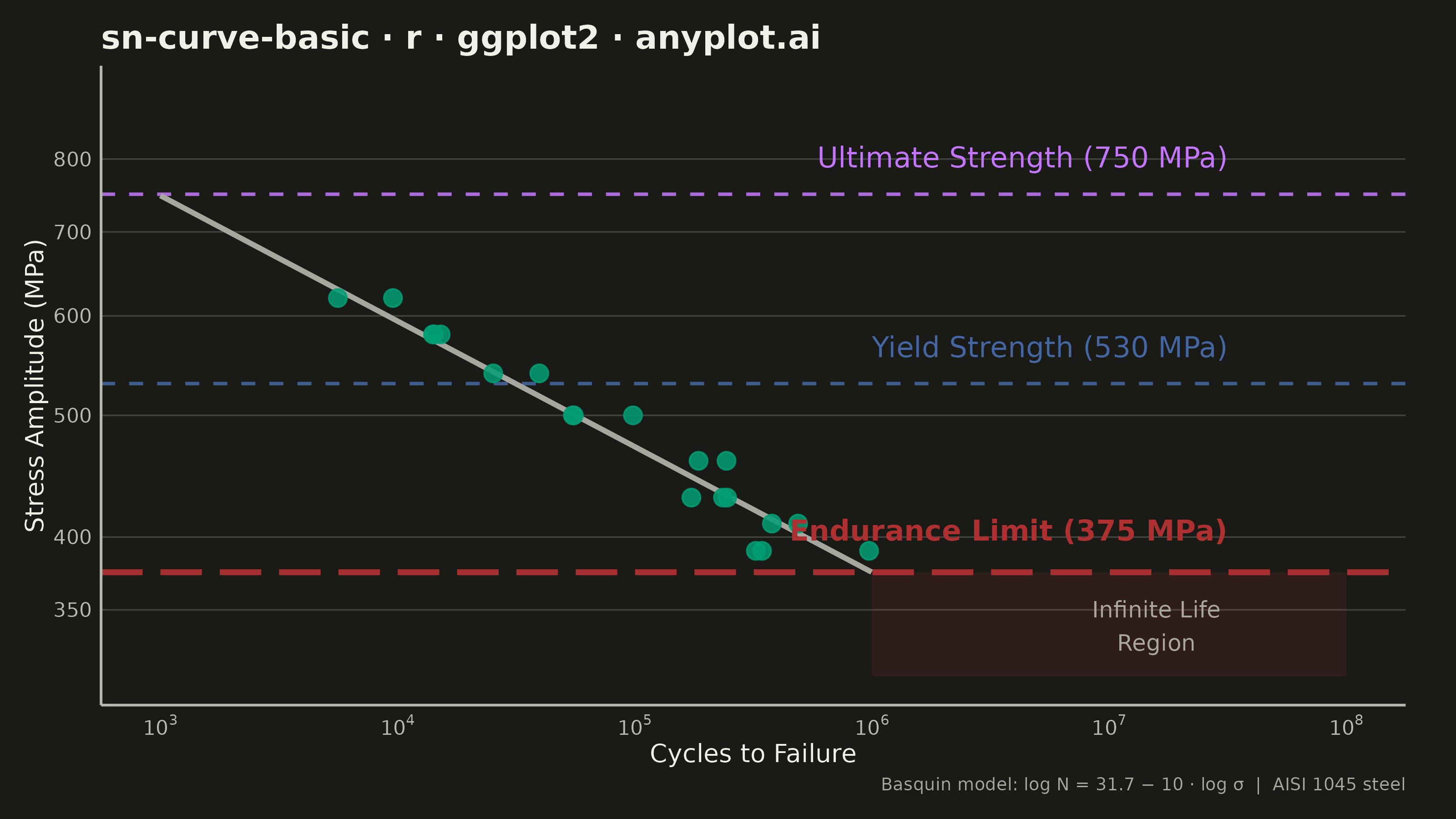
An S-N curve (also known as a Wöhler curve) visualizes the relationship between alternating stress amplitude and the number of cycles to failure for a material under fatigue loading. Both axes typically use logarithmic scales, with stress on the y-axis and cycle count on the x-axis. This plot is fundamental for predicting material fatigue life and identifying key material properties such as ultimate strength, yield strength, and endurance limit.
#' anyplot.ai
#' sn-curve-basic: S-N Curve (Wöhler Curve)
#' Library: ggplot2 3.5.1 | R 4.4.1
#' Quality: 89/100 | Created: 2026-05-20

library(ggplot2)
library(dplyr)
library(scales)
library(ragg)

set.seed(42)

# Theme tokens
THEME       <- Sys.getenv("ANYPLOT_THEME", "light")
PAGE_BG     <- if (THEME == "light") "#FAF8F1" else "#1A1A17"
INK         <- if (THEME == "light") "#1A1A17" else "#F0EFE8"
INK_SOFT    <- if (THEME == "light") "#4A4A44" else "#B8B7B0"
INK_MUTED   <- if (THEME == "light") "#6B6A63" else "#A8A79F"
IMPRINT   <- c("#009E73", "#C475FD", "#4467A3", "#BD8233",
                 "#AE3030", "#2ABCCD", "#954477")
GRID        <- adjustcolor(INK_SOFT, alpha.f = 0.25)

# AISI 1045 Steel material properties (MPa)
sigma_u <- 750   # Ultimate tensile strength
sigma_y <- 530   # Yield strength
sigma_e <- 375   # Endurance limit (~50% × UTS, engineering standard for steel)

# Basquin equation: log10(N) = C0 - k * log10(stress)
# C0 chosen so sigma_e maps to N ≈ 10^6 (conventional steel endurance life)
k  <- 10
C0 <- 31.74

# N at endurance limit — left boundary of infinite-life zone
N_endurance <- 10^(C0 - k * log10(sigma_e))

# Fatigue test specimens: multiple replicates per stress level (all above endurance limit)
stress_levels <- c(620, 580, 540, 500, 460, 430, 410, 390)
reps          <- c(2, 3, 2, 3, 2, 3, 2, 3)

df <- data.frame(stress = rep(stress_levels, reps)) |>
    mutate(cycles = 10^(C0 - k * log10(stress) + rnorm(n(), 0, 0.12)))

# Basquin fit line — log-spaced in cycle direction for accurate log-scale rendering
fit_df <- data.frame(
    cycles = 10^seq(3, log10(N_endurance * 0.998), length.out = 300)
) |> mutate(stress = 10^((C0 - log10(cycles)) / k))

# Plot
p <- ggplot() +
    # Infinite-life zone: stronger fill to emphasize key engineering insight
    annotate("rect",
        xmin = N_endurance, xmax = 10^8,
        ymin = 310, ymax = sigma_e,
        fill = IMPRINT[5], alpha = 0.14
    ) +
    # Reference lines for key material properties
    geom_hline(yintercept = sigma_u, linetype = "dashed",
               color = IMPRINT[2], linewidth = 0.65, alpha = 0.85) +
    geom_hline(yintercept = sigma_y, linetype = "dashed",
               color = IMPRINT[3], linewidth = 0.65, alpha = 0.85) +
    # Endurance limit thicker — the key design threshold for infinite life
    geom_hline(yintercept = sigma_e, linetype = "longdash",
               color = IMPRINT[5], linewidth = 1.1, alpha = 0.95) +
    # Basquin fit curve
    geom_line(data = fit_df, aes(x = cycles, y = stress),
              color = INK_MUTED, linewidth = 1.0) +
    # Test data scatter (multiple replicates per stress level)
    geom_point(data = df, aes(x = cycles, y = stress),
               shape = 21, size = 3.0, stroke = 0.5,
               color = IMPRINT[1], fill = IMPRINT[1], alpha = 0.85) +
    # Reference line labels — right-aligned at x = 10^7.5
    annotate("text", x = 10^7.5, y = sigma_u * 1.05,
             label = "Ultimate Strength (750 MPa)",
             color = IMPRINT[2], hjust = 1, vjust = 0, size = 4.0) +
    annotate("text", x = 10^7.5, y = sigma_y * 1.05,
             label = "Yield Strength (530 MPa)",
             color = IMPRINT[3], hjust = 1, vjust = 0, size = 4.0) +
    annotate("text", x = 10^7.5, y = sigma_e * 1.06,
             label = "Endurance Limit (375 MPa)",
             color = IMPRINT[5], hjust = 1, vjust = 0, size = 4.0,
             fontface = "bold") +
    # Infinite-life region label inside shaded zone
    annotate("text", x = 10^7.2, y = 340,
             label = "Infinite Life\nRegion",
             color = INK_MUTED, hjust = 0.5, size = 3.2, fontface = "italic") +
    # Log-log axes
    scale_x_log10(
        limits = c(1e3, 10^8),
        breaks = 10^(3:8),
        labels = scales::trans_format("log10", scales::math_format(10^.x))
    ) +
    scale_y_log10(
        limits = c(310, 900),
        breaks = c(350, 400, 500, 600, 700, 800),
        labels = scales::comma_format(accuracy = 1)
    ) +
    labs(
        title   = "sn-curve-basic · r · ggplot2 · anyplot.ai",
        x       = "Cycles to Failure",
        y       = "Stress Amplitude (MPa)",
        caption = "Basquin model: log N = 31.7 − 10 · log σ  |  AISI 1045 steel"
    ) +
    theme_minimal(base_size = 8) +
    theme(
        plot.background  = element_rect(fill = PAGE_BG, color = PAGE_BG),
        panel.background = element_rect(fill = PAGE_BG, color = NA),
        panel.grid.major.x = element_blank(),
        panel.grid.major.y = element_line(color = GRID, linewidth = 0.3),
        panel.grid.minor = element_blank(),
        panel.border     = element_blank(),
        axis.line        = element_line(color = INK_SOFT, linewidth = 0.5),
        axis.ticks       = element_blank(),
        axis.title       = element_text(color = INK, size = 10),
        axis.text        = element_text(color = INK_SOFT, size = 8),
        plot.title       = element_text(color = INK, size = 13, face = "bold"),
        plot.caption     = element_text(color = INK_MUTED, size = 7, hjust = 1),
        plot.margin      = margin(10, 20, 10, 10, "pt")
    )

# Save
ggsave(
    filename = sprintf("plot-%s.png", THEME),
    plot     = p,
    device   = ragg::agg_png,
    width    = 8,
    height   = 4.5,
    units    = "in",
    dpi      = 400
)
Runnable source as JSON, for any HTTP client: https://api.anyplot.ai/specs/sn-curve-basic/ggplot2/code. Any spec id and library id listed in llms-full.txt fit the same URL shape; every URL below is complete and callable.
{
  "spec_id": "sn-curve-basic",
  "language": "r",
  "library": "ggplot2",
  "page": "https://anyplot.ai/sn-curve-basic/r/ggplot2",
  "hub": "https://anyplot.ai/sn-curve-basic",
  "code_json": "https://api.anyplot.ai/specs/sn-curve-basic/ggplot2/code",
  "spec_json": "https://api.anyplot.ai/specs/sn-curve-basic",
  "render_light_png": "https://storage.googleapis.com/anyplot-images/plots/sn-curve-basic/r/ggplot2/plot-light.png",
  "render_dark_png": "https://storage.googleapis.com/anyplot-images/plots/sn-curve-basic/r/ggplot2/plot-dark.png",
  "quality_score": 89.0,
  "license": "MIT",
  "guide": "https://anyplot.ai/llms.txt"
}
Part of S-N Curve (Wöhler Curve) on anyplot.ai.