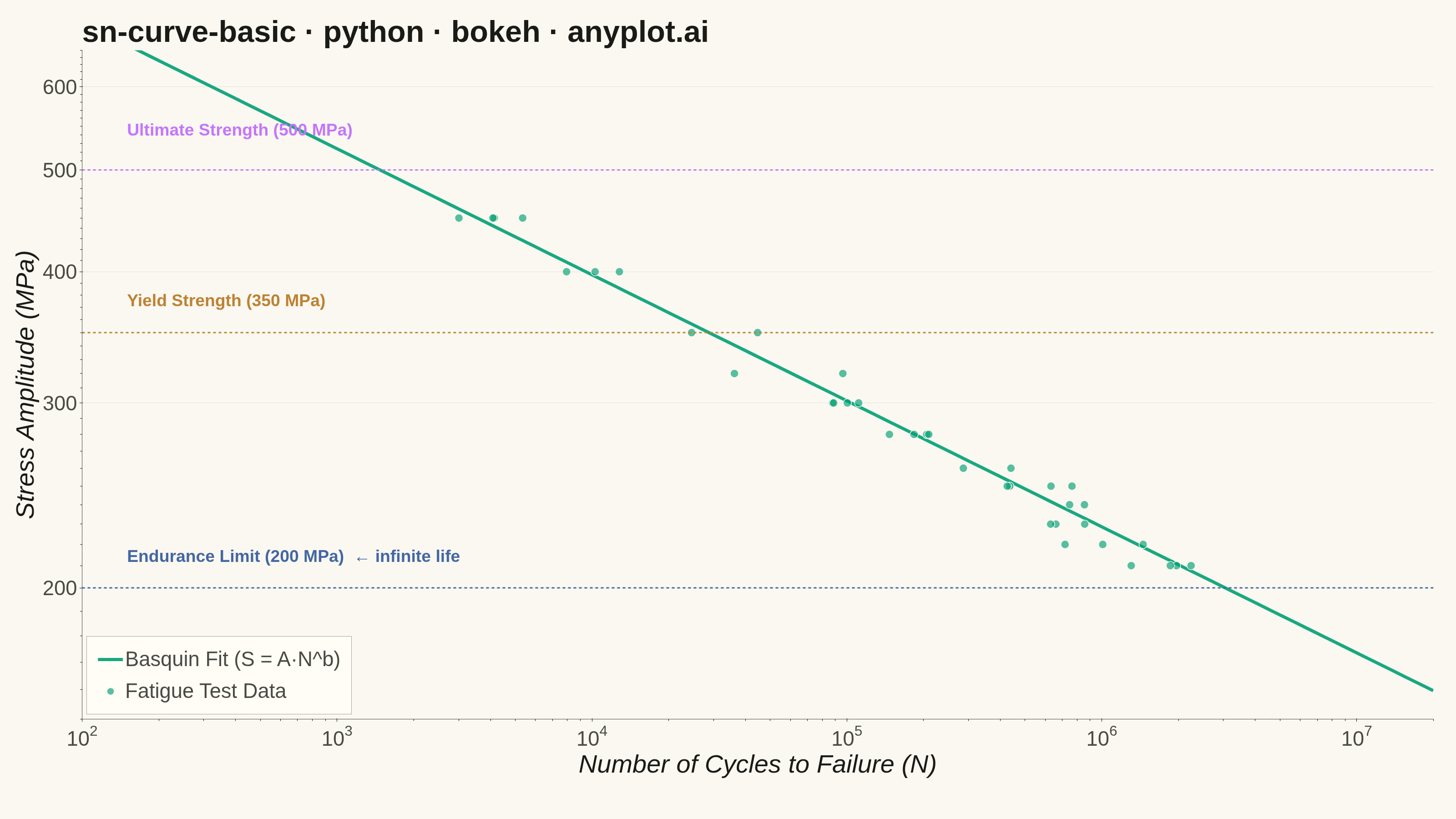
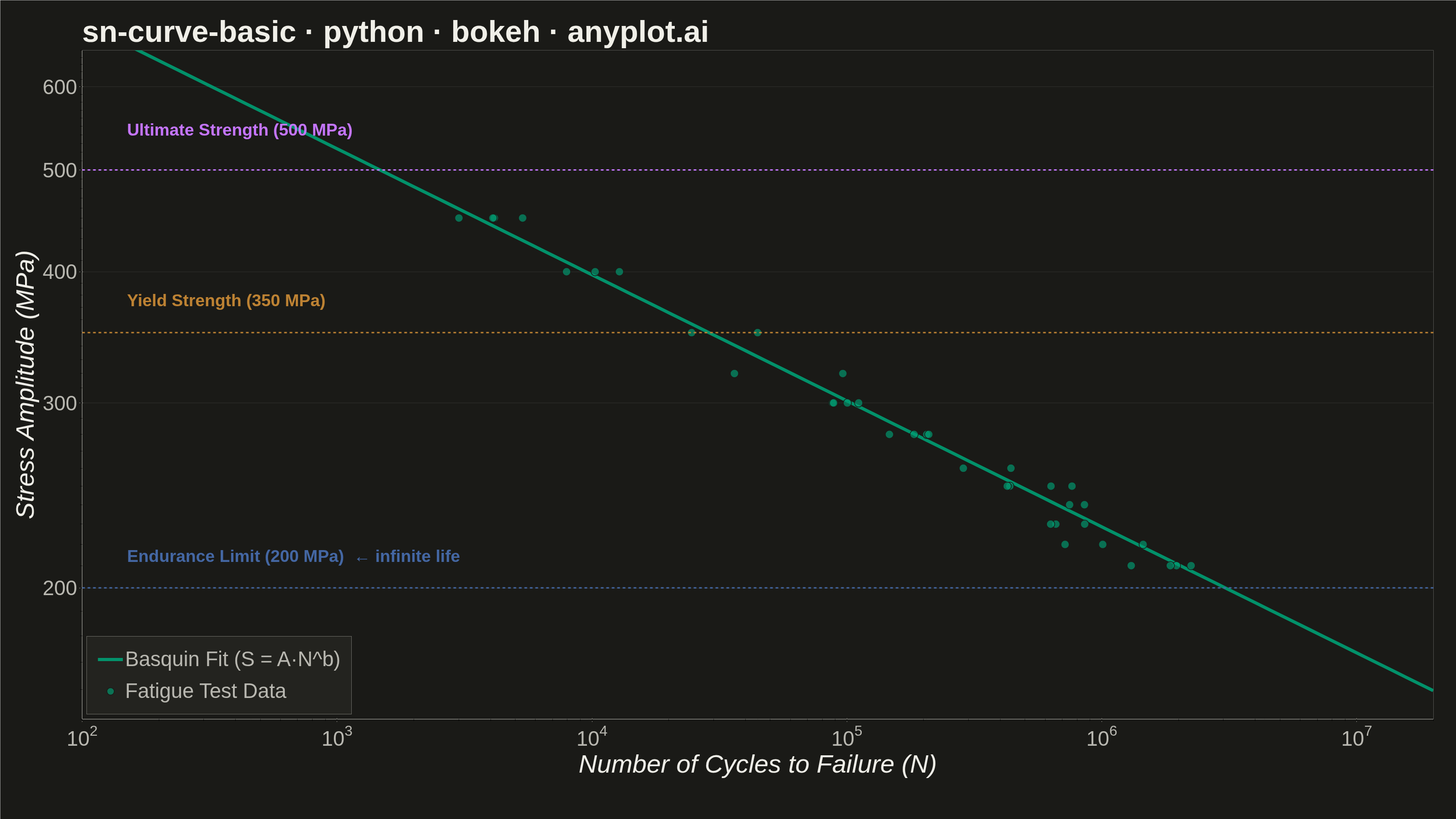
An S-N curve (also known as a Wöhler curve) visualizes the relationship between alternating stress amplitude and the number of cycles to failure for a material under fatigue loading. Both axes typically use logarithmic scales, with stress on the y-axis and cycle count on the x-axis. This plot is fundamental for predicting material fatigue life and identifying key material properties such as ultimate strength, yield strength, and endurance limit.
""" anyplot.ai
sn-curve-basic: S-N Curve (Wöhler Curve)
Library: bokeh 3.9.0 | Python 3.13.13
Quality: 92/100 | Updated: 2026-05-20
"""

import os
import sys
import time
from pathlib import Path


# Remove the current directory from sys.path to avoid circular imports with bokeh.py
sys.path = [p for p in sys.path if p not in ("", ".", os.getcwd(), os.path.dirname(__file__))]

import numpy as np
from bokeh.io import output_file, save
from bokeh.models import BoxAnnotation, ColumnDataSource, HoverTool, Label, Span
from bokeh.plotting import figure
from selenium import webdriver
from selenium.webdriver.chrome.options import Options


THEME = os.getenv("ANYPLOT_THEME", "light")
PAGE_BG = "#FAF8F1" if THEME == "light" else "#1A1A17"
ELEVATED_BG = "#FFFDF6" if THEME == "light" else "#242420"
INK = "#1A1A17" if THEME == "light" else "#F0EFE8"
INK_SOFT = "#4A4A44" if THEME == "light" else "#B8B7B0"

BRAND = "#009E73"  # Okabe-Ito position 1 — data series
ULT_COLOR = "#C475FD"  # Okabe-Ito position 2 — Ultimate Strength line
ENDU_COLOR = "#4467A3"  # Okabe-Ito position 3 — Endurance Limit line
YIELD_COLOR = "#BD8233"  # Okabe-Ito position 4 — Yield Strength line

# Data — S-N fatigue test results for steel specimens (Basquin equation)
np.random.seed(42)

A = 1200  # MPa coefficient
b = -0.12  # Basquin exponent

stress_levels = np.array([450, 400, 350, 320, 300, 280, 260, 250, 240, 230, 220, 210])

cycles_list = []
stress_list = []

for stress_val in stress_levels:
    N_theoretical = (stress_val / A) ** (1 / b)
    n_specimens = np.random.randint(2, 5)
    scatter = np.random.lognormal(0, 0.3, n_specimens)
    cycles_actual = N_theoretical * scatter
    cycles_list.extend(cycles_actual)
    stress_list.extend([stress_val] * n_specimens)

cycles = np.array(cycles_list)
stress = np.array(stress_list)

ultimate_strength = 500  # MPa
yield_strength = 350  # MPa
endurance_limit = 200  # MPa

cycles_fit = np.logspace(2, 7.3, 100)
stress_fit = A * (cycles_fit**b)

source = ColumnDataSource(data={"cycles": cycles, "stress": stress})
source_fit = ColumnDataSource(data={"cycles_fit": cycles_fit, "stress_fit": stress_fit})

# Plot
p = figure(
    width=3200,
    height=1800,
    title="sn-curve-basic · python · bokeh · anyplot.ai",
    x_axis_label="Number of Cycles to Failure (N)",
    y_axis_label="Stress Amplitude (MPa)",
    x_axis_type="log",
    y_axis_type="log",
    y_range=(150, 650),
    x_range=(100, 2e7),
    toolbar_location=None,
    min_border_bottom=220,
    min_border_left=180,
    min_border_top=110,
    min_border_right=50,
)

# Infinite-life zone shaded below the endurance limit
p.add_layout(BoxAnnotation(top=endurance_limit, bottom=0, fill_color=ENDU_COLOR, fill_alpha=0.12, line_color=None))

p.line(
    x="cycles_fit",
    y="stress_fit",
    source=source_fit,
    line_width=7,
    line_color=BRAND,
    line_alpha=0.9,
    legend_label="Basquin Fit (S = A·N^b)",
)

p.scatter(
    x="cycles",
    y="stress",
    source=source,
    size=18,
    fill_color=BRAND,
    fill_alpha=0.65,
    line_color=PAGE_BG,
    line_width=1.5,
    legend_label="Fatigue Test Data",
)

hover = HoverTool(tooltips=[("Cycles to Failure", "@cycles{0.00e+0}"), ("Stress Amplitude", "@stress{0} MPa")])
p.add_tools(hover)

# Reference lines for material properties
p.add_layout(
    Span(location=ultimate_strength, dimension="width", line_color=ULT_COLOR, line_width=3, line_dash="dashed")
)
p.add_layout(Span(location=yield_strength, dimension="width", line_color=YIELD_COLOR, line_width=3, line_dash="dashed"))
p.add_layout(Span(location=endurance_limit, dimension="width", line_color=ENDU_COLOR, line_width=3, line_dash="dashed"))

p.add_layout(
    Label(
        x=150,
        y=535,
        text=f"Ultimate Strength ({ultimate_strength} MPa)",
        text_font_size="28pt",
        text_color=ULT_COLOR,
        text_font_style="bold",
    )
)
p.add_layout(
    Label(
        x=150,
        y=368,
        text=f"Yield Strength ({yield_strength} MPa)",
        text_font_size="28pt",
        text_color=YIELD_COLOR,
        text_font_style="bold",
    )
)
p.add_layout(
    Label(
        x=150,
        y=210,
        text=f"Endurance Limit ({endurance_limit} MPa)  ← infinite life",
        text_font_size="28pt",
        text_color=ENDU_COLOR,
        text_font_style="bold",
    )
)

# Style — font sizes per default-style-guide.md "Visual Sizing Defaults" for bokeh
p.title.text_font_size = "50pt"
p.title.text_color = INK
p.xaxis.axis_label_text_font_size = "42pt"
p.yaxis.axis_label_text_font_size = "42pt"
p.xaxis.axis_label_text_color = INK
p.yaxis.axis_label_text_color = INK
p.xaxis.major_label_text_font_size = "34pt"
p.yaxis.major_label_text_font_size = "34pt"
p.xaxis.major_label_text_color = INK_SOFT
p.yaxis.major_label_text_color = INK_SOFT
p.xaxis.axis_line_color = INK_SOFT
p.yaxis.axis_line_color = INK_SOFT
p.xaxis.major_tick_line_color = INK_SOFT
p.yaxis.major_tick_line_color = INK_SOFT

# Y-only grid for cleaner line+scatter chart
p.xgrid.grid_line_color = None
p.ygrid.grid_line_color = INK
p.ygrid.grid_line_alpha = 0.10

p.background_fill_color = PAGE_BG
p.border_fill_color = PAGE_BG
p.outline_line_color = None

p.legend.location = "bottom_left"
p.legend.label_text_font_size = "34pt"
p.legend.label_text_color = INK_SOFT
p.legend.background_fill_color = ELEVATED_BG
p.legend.border_line_color = INK_SOFT
p.legend.glyph_width = 55
p.legend.glyph_height = 40
p.legend.spacing = 18
p.legend.padding = 24

# Save HTML
output_file(f"plot-{THEME}.html")
save(p)

# Save PNG via headless Chrome (Selenium)
W, H = 3200, 1800
opts = Options()
for arg in (
    "--headless=new",
    "--no-sandbox",
    "--disable-dev-shm-usage",
    "--disable-gpu",
    f"--window-size={W},{H}",
    "--hide-scrollbars",
):
    opts.add_argument(arg)

driver = webdriver.Chrome(options=opts)
# Override emulated viewport to exactly W×H regardless of browser chrome overhead
driver.execute_cdp_cmd(
    "Emulation.setDeviceMetricsOverride", {"width": W, "height": H, "deviceScaleFactor": 1, "mobile": False}
)
driver.get(f"file://{Path(f'plot-{THEME}.html').resolve()}")
time.sleep(3)
driver.save_screenshot(f"plot-{THEME}.png")
driver.quit()
Runnable source as JSON, for any HTTP client: https://api.anyplot.ai/specs/sn-curve-basic/bokeh/code. Any spec id and library id listed in llms-full.txt fit the same URL shape; every URL below is complete and callable.
{
  "spec_id": "sn-curve-basic",
  "language": "python",
  "library": "bokeh",
  "page": "https://anyplot.ai/sn-curve-basic/python/bokeh",
  "hub": "https://anyplot.ai/sn-curve-basic",
  "code_json": "https://api.anyplot.ai/specs/sn-curve-basic/bokeh/code",
  "spec_json": "https://api.anyplot.ai/specs/sn-curve-basic",
  "render_light_png": "https://storage.googleapis.com/anyplot-images/plots/sn-curve-basic/python/bokeh/plot-light.png",
  "render_dark_png": "https://storage.googleapis.com/anyplot-images/plots/sn-curve-basic/python/bokeh/plot-dark.png",
  "interactive_light_html": "https://storage.googleapis.com/anyplot-images/plots/sn-curve-basic/python/bokeh/plot-light.html",
  "interactive_dark_html": "https://storage.googleapis.com/anyplot-images/plots/sn-curve-basic/python/bokeh/plot-dark.html",
  "quality_score": 92.0,
  "license": "MIT",
  "guide": "https://anyplot.ai/llms.txt"
}
Part of S-N Curve (Wöhler Curve) on anyplot.ai.