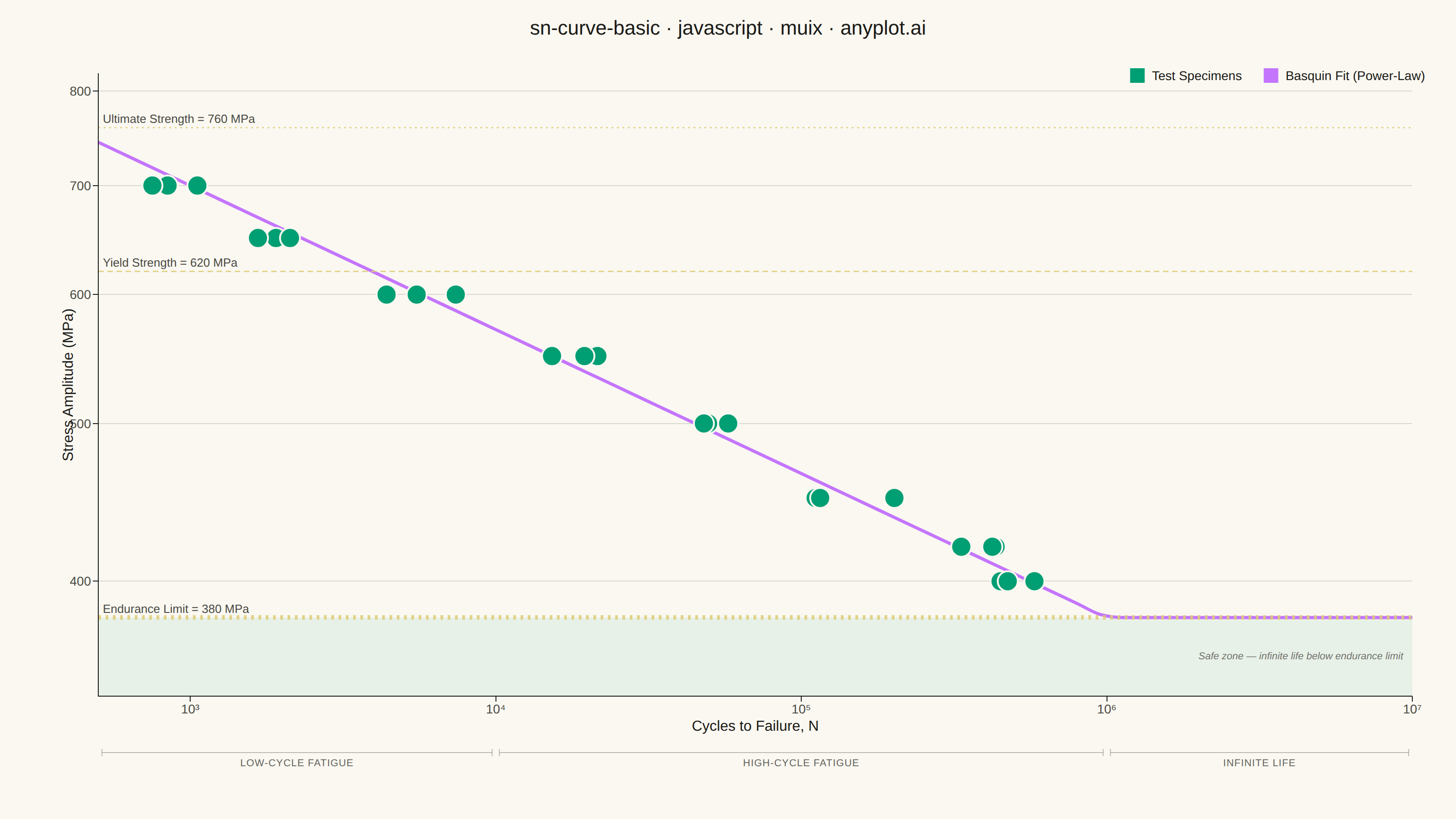
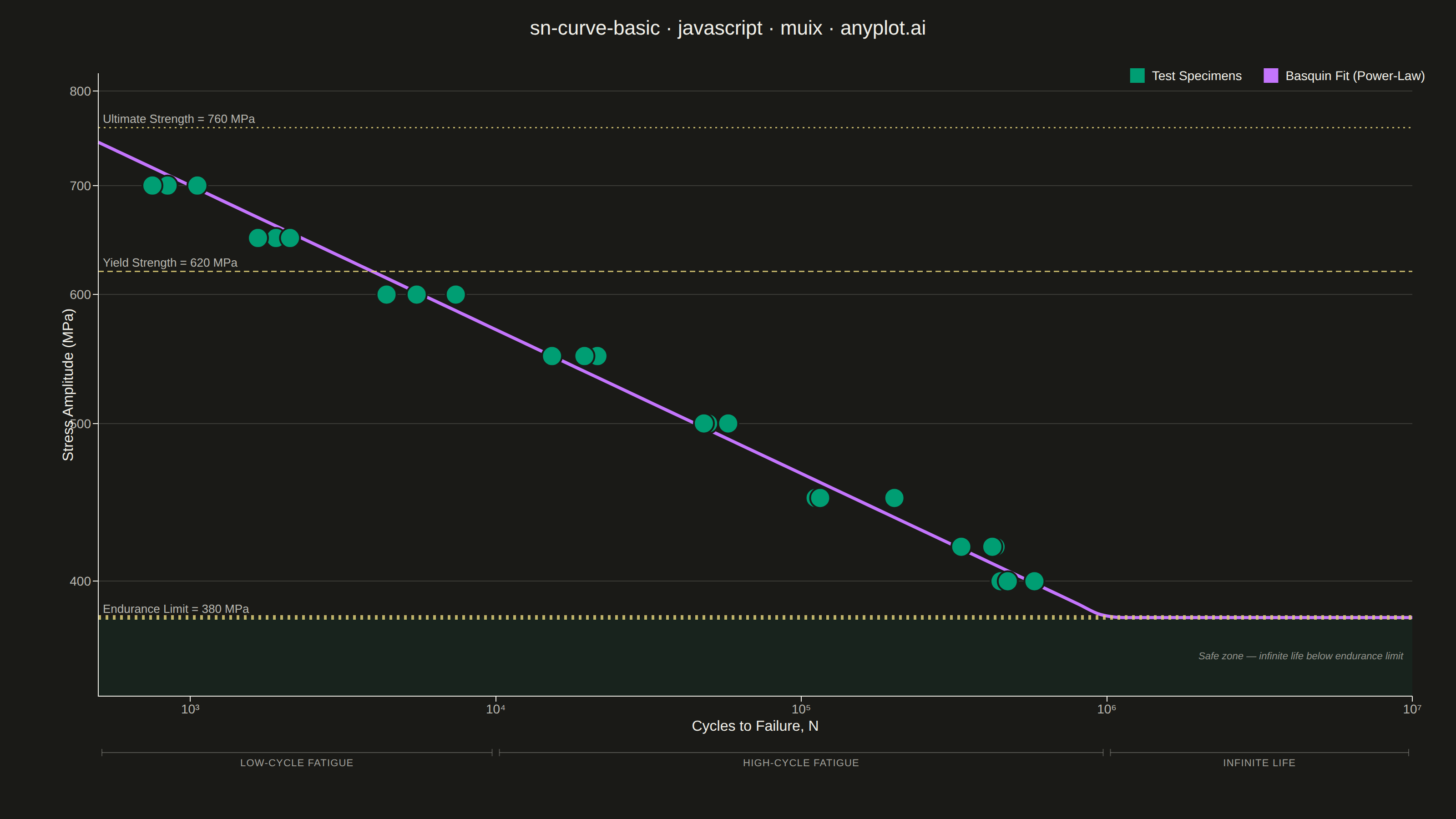
The same plot in 14 other libraries — JavaScript: Chart.js, D3.js, Apache ECharts, Highcharts; Python: Altair, Bokeh, lets-plot, Matplotlib, Plotly, plotnine, Pygal, Seaborn; R: ggplot2; Julia: Makie.jl. Compare all 15 side by side: S-N Curve (Wöhler Curve) in Python, R, Julia and JavaScript.
An S-N curve (also known as a Wöhler curve) visualizes the relationship between alternating stress amplitude and the number of cycles to failure for a material under fatigue loading. Both axes typically use logarithmic scales, with stress on the y-axis and cycle count on the x-axis. This plot is fundamental for predicting material fatigue life and identifying key material properties such as ultimate strength, yield strength, and endurance limit.
// anyplot.ai
// sn-curve-basic: S-N Curve (Wöhler Curve)
// Library: muix 7.29.1 | JavaScript 22.23.2
// Quality: 86/100 | Created: 2026-09-02

import * as React from "react";
import { ChartContainer } from "@mui/x-charts/ChartContainer";
import { LinePlot } from "@mui/x-charts/LineChart";
import { ScatterPlot } from "@mui/x-charts/ScatterChart";
import { ChartsXAxis } from "@mui/x-charts/ChartsXAxis";
import { ChartsYAxis } from "@mui/x-charts/ChartsYAxis";
import { ChartsGrid } from "@mui/x-charts/ChartsGrid";
import { ChartsLegend } from "@mui/x-charts/ChartsLegend";
import { ChartsReferenceLine } from "@mui/x-charts/ChartsReferenceLine";
import { ChartsTooltip } from "@mui/x-charts/ChartsTooltip";
import { useDrawingArea, useXScale, useYScale } from "@mui/x-charts/hooks";
import Box from "@mui/material/Box";
import Typography from "@mui/material/Typography";

const t = window.ANYPLOT_TOKENS;

// --- Basquin power-law fit, anchored between a low-cycle point and the knee
// where the curve levels off at the endurance limit: S = C * N^b -----------
const N1 = 1e3;
const S1 = 700; // MPa, low-cycle anchor
const N_KNEE = 1e6; // cycles — transition from finite life to infinite life
const ENDURANCE_LIMIT = 380; // MPa — safe stress below which failure won't occur
const ULTIMATE_STRENGTH = 760; // MPa
const YIELD_STRENGTH = 620; // MPa

const B_EXP = Math.log(ENDURANCE_LIMIT / S1) / Math.log(N_KNEE / N1);
const C_COEF = S1 * Math.pow(N1, -B_EXP);
const basquinStress = (n) =>
  n <= N_KNEE ? C_COEF * Math.pow(n, B_EXP) : ENDURANCE_LIMIT;
const basquinCycles = (s) => Math.pow(s / C_COEF, 1 / B_EXP);

// --- Fitted curve: dense log-spaced grid from low-cycle fatigue through the
// knee into the infinite-life region -----------------------------------------
const X_MIN = 500;
const X_MAX = 1e7;
const GRID_N = 60;
const logMin = Math.log10(X_MIN);
const logMax = Math.log10(X_MAX);
const fitCycles = Array.from({ length: GRID_N }, (_, i) =>
  Math.pow(10, logMin + (i / (GRID_N - 1)) * (logMax - logMin)),
);
const fitStress = fitCycles.map(basquinStress);

// --- Test specimens: fixed stress per level, scatter in life (cycles) — the
// standard convention for fatigue coupon testing ----------------------------
let seed = 42;
function rng() {
  seed = (Math.imul(1664525, seed) + 1013904223) >>> 0;
  return seed / 4294967296;
}

const STRESS_LEVELS = [700, 650, 600, 550, 500, 450, 420, 400];
const SPECIMENS_PER_LEVEL = 3;
const specimens = [];
STRESS_LEVELS.forEach((stress, levelIdx) => {
  const baseCycles = basquinCycles(stress);
  for (let k = 0; k < SPECIMENS_PER_LEVEL; k++) {
    const jitter = Math.pow(10, (rng() - 0.5) * 0.3);
    specimens.push({
      id: `L${levelIdx}-${k}`,
      x: Math.round(baseCycles * jitter),
      y: stress,
    });
  }
});

// --- Axis formatting ---------------------------------------------------------
const SUPERSCRIPT = {
  "0": "⁰",
  "1": "¹",
  "2": "²",
  "3": "³",
  "4": "⁴",
  "5": "⁵",
  "6": "⁶",
  "7": "⁷",
  "8": "⁸",
  "9": "⁹",
};
const fmtCycles = (n) => {
  const exp = Math.round(Math.log10(n));
  return `10${String(exp)
    .split("")
    .map((d) => SUPERSCRIPT[d])
    .join("")}`;
};
const CYCLE_TICKS = [1e3, 1e4, 1e5, 1e6, 1e7];
const STRESS_TICKS = [400, 500, 600, 700, 800];

const TITLE = "sn-curve-basic · javascript · muix · anyplot.ai";

// --- Fatigue life regions, called out in the spec notes: low-cycle (plastic),
// high-cycle (elastic), and infinite-life (below the endurance limit) ---------
const LOW_HIGH_BOUNDARY = 1e4; // conventional low-cycle / high-cycle divide
const REGIONS = [
  { label: "LOW-CYCLE FATIGUE", xMin: X_MIN, xMax: LOW_HIGH_BOUNDARY },
  { label: "HIGH-CYCLE FATIGUE", xMin: LOW_HIGH_BOUNDARY, xMax: N_KNEE },
  { label: "INFINITE LIFE", xMin: N_KNEE, xMax: X_MAX },
];

// Translucent band below the endurance limit — the "safe for infinite life"
// stress range — plus a thicker, amber-colored endurance-limit stroke so it
// stays visually distinct from the purple fit line where the two coincide.
function SafeZoneBand() {
  const { left, top, width, height } = useDrawingArea();
  const yScale = useYScale("stress") as ((v: number) => number) | undefined;
  if (!yScale) return null;
  const yTop = yScale(ENDURANCE_LIMIT);
  const yBottom = top + height;
  return (
    <g>
      <rect
        x={left}
        y={yTop}
        width={width}
        height={Math.max(yBottom - yTop, 1)}
        fill={t.palette[0]}
        opacity={0.07}
      />
      <text
        x={left + width - 10}
        y={yTop + (yBottom - yTop) / 2}
        textAnchor="end"
        dominantBaseline="middle"
        fontSize={11}
        fontStyle="italic"
        fill={t.inkSoft}
        opacity={0.75}
      >
        Safe zone — infinite life below endurance limit
      </text>
    </g>
  );
}

// Region labels + boundary ticks placed under the x-axis, calling out the
// three fatigue regions described in the spec (low-cycle / high-cycle /
// infinite-life) so the story reads without parsing the reference-line labels.
function FatigueRegionLabels() {
  const { left, top, width, height } = useDrawingArea();
  const xScale = useXScale("cycles") as ((v: number) => number) | undefined;
  if (!xScale) return null;
  const lineY = top + height + 62;
  const textY = lineY + 15;
  return (
    <g>
      {REGIONS.map((r) => {
        const x0 = xScale(Math.max(r.xMin, X_MIN));
        const x1 = xScale(Math.min(r.xMax, X_MAX));
        const xMid = (x0 + x1) / 2;
        return (
          <React.Fragment key={r.label}>
            <line
              x1={x0 + 4}
              y1={lineY}
              x2={x1 - 4}
              y2={lineY}
              stroke={t.inkSoft}
              strokeWidth={1}
              opacity={0.35}
            />
            <line
              x1={x0 + 4}
              y1={lineY - 4}
              x2={x0 + 4}
              y2={lineY + 4}
              stroke={t.inkSoft}
              strokeWidth={1}
              opacity={0.35}
            />
            <line
              x1={x1 - 4}
              y1={lineY - 4}
              x2={x1 - 4}
              y2={lineY + 4}
              stroke={t.inkSoft}
              strokeWidth={1}
              opacity={0.35}
            />
            <text
              x={xMid}
              y={textY}
              textAnchor="middle"
              fontSize={11}
              letterSpacing={0.6}
              fill={t.inkSoft}
              opacity={0.85}
            >
              {r.label}
            </text>
          </React.Fragment>
        );
      })}
    </g>
  );
}

export default function Chart() {
  const { width, height } = window.ANYPLOT_SIZE;
  const TITLE_H = 56;
  const chartH = height - TITLE_H;

  return (
    <Box
      sx={{
        width,
        height,
        background: t.pageBg,
        display: "flex",
        flexDirection: "column",
      }}
    >
      <Typography
        sx={{
          fontSize: "22px",
          fontWeight: 500,
          color: t.ink,
          textAlign: "center",
          pt: "14px",
          pb: "6px",
        }}
      >
        {TITLE}
      </Typography>
      <ChartContainer
        width={width}
        height={chartH}
        margin={{ top: 28, right: 48, bottom: 132, left: 108 }}
        sx={{
          ".MuiLineElement-series-fit": { strokeWidth: 3.5 },
          "& circle": { stroke: t.pageBg, strokeWidth: 2 },
        }}
        series={[
          {
            type: "scatter",
            id: "specimens",
            xAxisId: "cycles",
            yAxisId: "stress",
            data: specimens,
            color: t.palette[0],
            markerSize: 11,
            label: "Test Specimens",
          },
          {
            type: "line",
            id: "fit",
            xAxisId: "cycles",
            yAxisId: "stress",
            data: fitStress,
            color: t.palette[1],
            showMark: false,
            curve: "monotoneX",
            label: "Basquin Fit (Power-Law)",
          },
        ]}
        xAxis={[
          {
            id: "cycles",
            scaleType: "log",
            data: fitCycles,
            min: X_MIN,
            max: X_MAX,
            label: "Cycles to Failure, N",
            valueFormatter: fmtCycles,
            tickInterval: CYCLE_TICKS,
            tickLabelStyle: { fontSize: 14, fill: t.inkSoft },
            labelStyle: { fontSize: 16, fill: t.ink },
          },
        ]}
        yAxis={[
          {
            id: "stress",
            scaleType: "log",
            min: 340,
            max: 820,
            label: "Stress Amplitude (MPa)",
            tickInterval: STRESS_TICKS,
            tickLabelStyle: { fontSize: 14, fill: t.inkSoft },
            labelStyle: { fontSize: 16, fill: t.ink },
          },
        ]}
      >
        <ChartsGrid horizontal />
        <SafeZoneBand />
        <LinePlot skipAnimation />
        <ScatterPlot skipAnimation />
        <ChartsReferenceLine
          y={ULTIMATE_STRENGTH}
          axisId="stress"
          label={`Ultimate Strength = ${ULTIMATE_STRENGTH} MPa`}
          labelAlign="start"
          labelStyle={{ fill: t.inkSoft, fontSize: 13 }}
          lineStyle={{
            stroke: t.amber,
            strokeDasharray: "2 4",
            strokeWidth: 1.5,
            opacity: 0.85,
          }}
        />
        <ChartsReferenceLine
          y={YIELD_STRENGTH}
          axisId="stress"
          label={`Yield Strength = ${YIELD_STRENGTH} MPa`}
          labelAlign="start"
          labelStyle={{ fill: t.inkSoft, fontSize: 13 }}
          lineStyle={{
            stroke: t.amber,
            strokeDasharray: "6 4",
            strokeWidth: 1.5,
            opacity: 0.85,
          }}
        />
        <ChartsReferenceLine
          y={ENDURANCE_LIMIT}
          axisId="stress"
          label={`Endurance Limit = ${ENDURANCE_LIMIT} MPa`}
          labelAlign="start"
          labelStyle={{ fill: t.inkSoft, fontSize: 13 }}
          lineStyle={{
            stroke: t.amber,
            strokeDasharray: "3 5",
            strokeWidth: 5,
            opacity: 0.85,
          }}
        />
        <ChartsXAxis axisId="cycles" />
        <ChartsYAxis axisId="stress" />
        <ChartsLegend
          position={{ vertical: "top", horizontal: "right" }}
          slotProps={{
            legend: {
              itemMarkWidth: 16,
              itemMarkHeight: 16,
              markGap: 8,
              itemGap: 24,
              labelStyle: { fontSize: 14, fill: t.ink },
            },
          }}
        />
        <ChartsTooltip trigger="item" />
        <FatigueRegionLabels />
      </ChartContainer>
    </Box>
  );
}
Runnable source as JSON, for any HTTP client: https://api.anyplot.ai/specs/sn-curve-basic/muix/code. Any spec id and library id listed in llms-full.txt fit the same URL shape; every URL below is complete and callable.
{
  "spec_id": "sn-curve-basic",
  "language": "javascript",
  "library": "muix",
  "page": "https://anyplot.ai/sn-curve-basic/javascript/muix",
  "hub": "https://anyplot.ai/sn-curve-basic",
  "code_json": "https://api.anyplot.ai/specs/sn-curve-basic/muix/code",
  "spec_json": "https://api.anyplot.ai/specs/sn-curve-basic",
  "render_light_png": "https://storage.googleapis.com/anyplot-images/plots/sn-curve-basic/javascript/muix/plot-light.png",
  "render_dark_png": "https://storage.googleapis.com/anyplot-images/plots/sn-curve-basic/javascript/muix/plot-dark.png",
  "interactive_light_html": "https://storage.googleapis.com/anyplot-images/plots/sn-curve-basic/javascript/muix/plot-light.html",
  "interactive_dark_html": "https://storage.googleapis.com/anyplot-images/plots/sn-curve-basic/javascript/muix/plot-dark.html",
  "quality_score": 86.0,
  "license": "MIT",
  "guide": "https://anyplot.ai/llms.txt"
}
Part of S-N Curve (Wöhler Curve) on anyplot.ai.