The same plot in 14 other libraries — JavaScript: Chart.js, D3.js, Apache ECharts, MUI X Charts; Python: Altair, Bokeh, lets-plot, Matplotlib, Plotly, plotnine, Pygal, Seaborn; R: ggplot2; Julia: Makie.jl. Compare all 15 side by side: S-N Curve (Wöhler Curve) in Python, R, Julia and JavaScript.
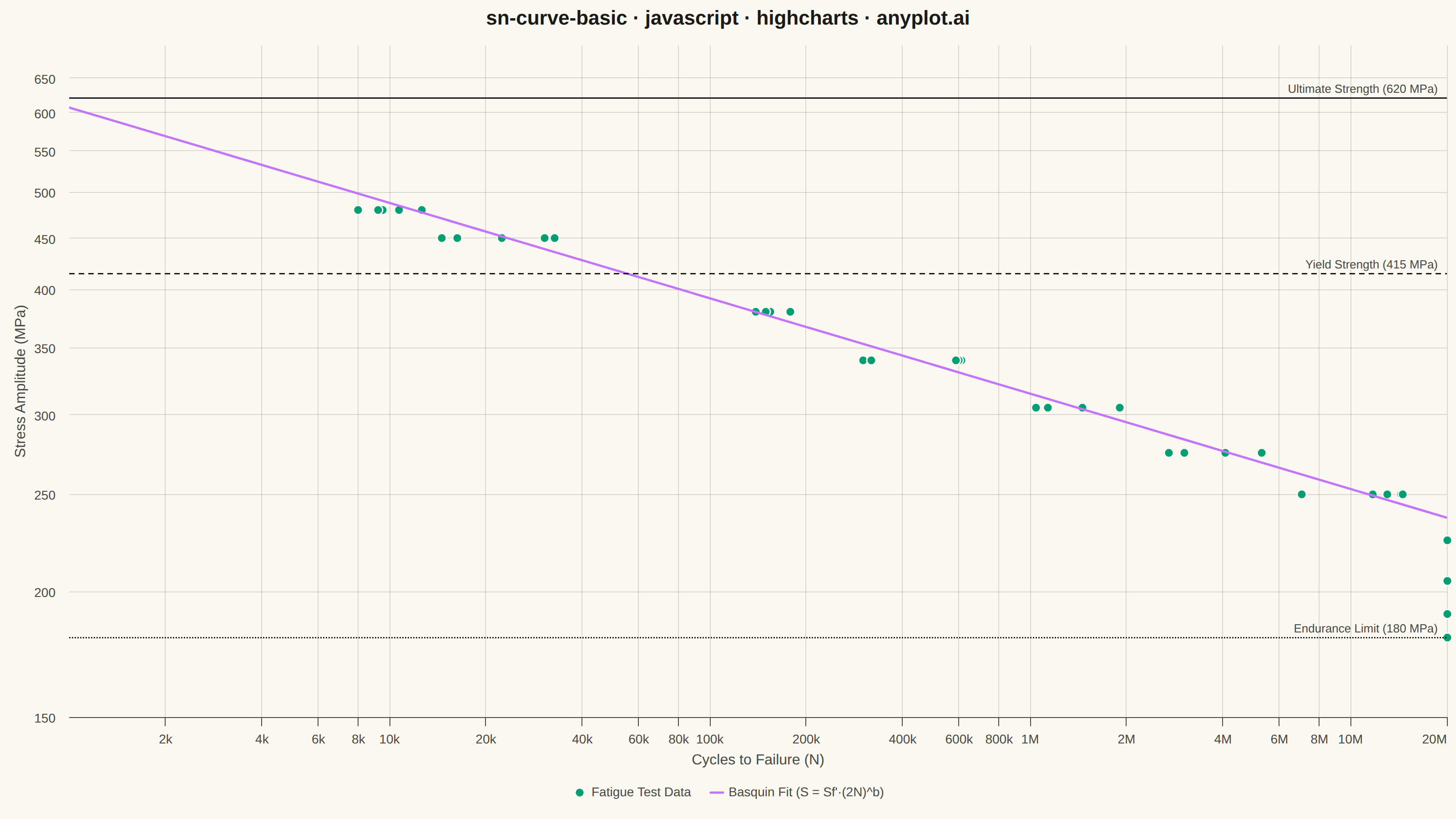
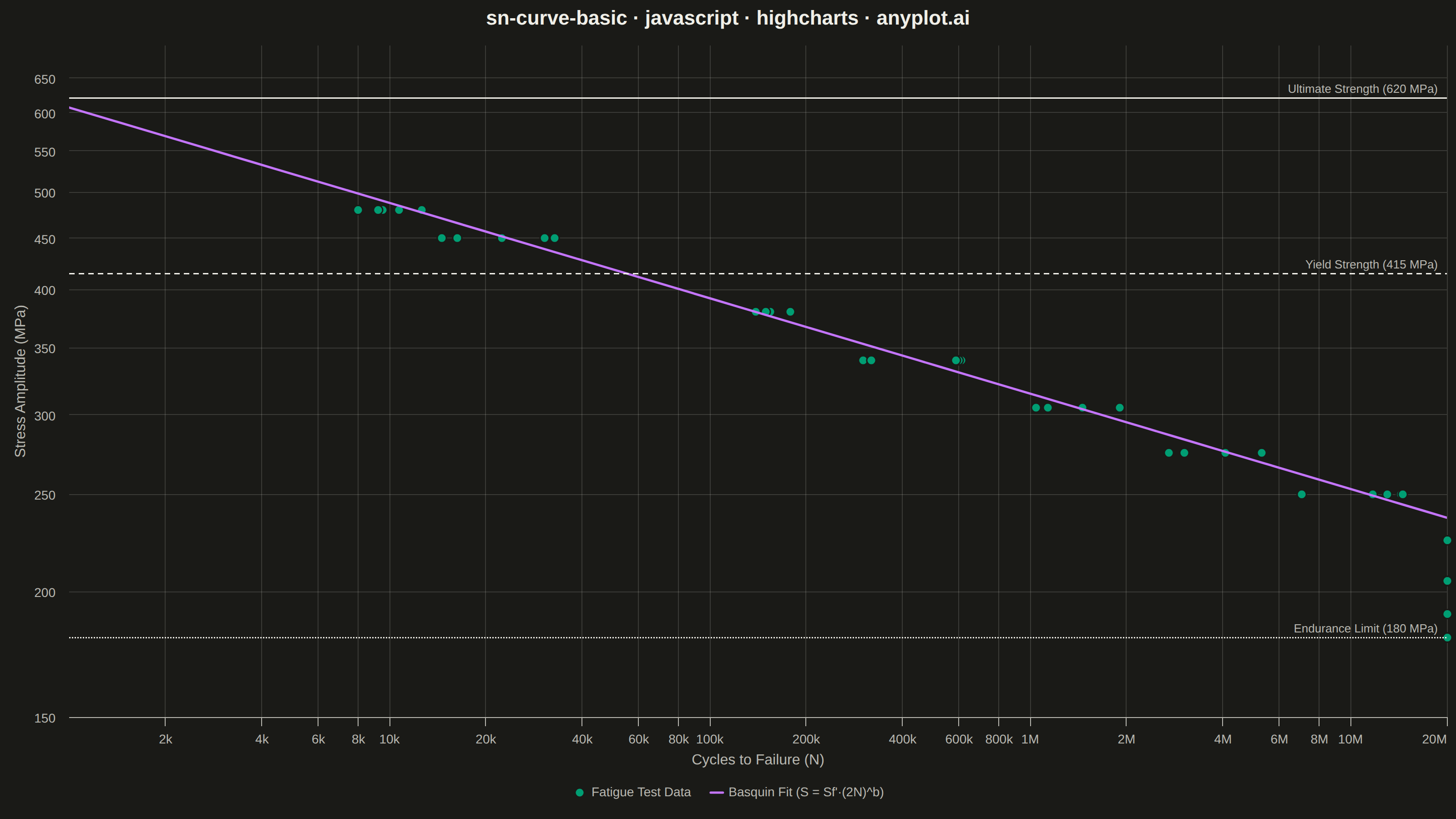
An S-N curve (also known as a Wöhler curve) visualizes the relationship between alternating stress amplitude and the number of cycles to failure for a material under fatigue loading. Both axes typically use logarithmic scales, with stress on the y-axis and cycle count on the x-axis. This plot is fundamental for predicting material fatigue life and identifying key material properties such as ultimate strength, yield strength, and endurance limit.
// anyplot.ai
// sn-curve-basic: S-N Curve (Wöhler Curve)
// Library: highcharts 12.6.0 | JavaScript 22.23.2
// Quality: 91/100 | Created: 2026-09-02

const t = window.ANYPLOT_TOKENS;

// --- Data (in-memory, deterministic) ----------------------------------------
// Fixed-seed LCG — the browser has no seeded RNG.
function lcg(seed) {
  let state = seed;
  return function () {
    state = (state * 1664525 + 1013904223) % 4294967296;
    return state / 4294967296;
  };
}
const rand = lcg(42);

// Basquin's law for a steel alloy: stress = Sf' * (2N)^b
const FATIGUE_STRENGTH_COEFF = 1250; // Sf', MPa
const FATIGUE_STRENGTH_EXP = -0.095; // b
const ULTIMATE_STRENGTH = 620; // MPa
const YIELD_STRENGTH = 415; // MPa
const ENDURANCE_LIMIT = 180; // MPa — asymptote for infinite life
const RUNOUT_CYCLES = 2e7; // test termination — specimens beyond this are "runouts"

function cyclesForStress(stress) {
  return 0.5 * Math.pow(stress / FATIGUE_STRENGTH_COEFF, 1 / FATIGUE_STRENGTH_EXP);
}
function stressForCycles(cycles) {
  return Math.max(FATIGUE_STRENGTH_COEFF * Math.pow(2 * cycles, FATIGUE_STRENGTH_EXP), ENDURANCE_LIMIT);
}

// Test specimens at 11 stress levels, 5 specimens each (steel coupon fatigue tests).
// The top two levels (480, 450 MPa) sit above yield strength, giving the
// low-cycle/plastic region alongside the high-cycle/elastic and infinite-life ones.
const stressLevels = [480, 450, 380, 340, 305, 275, 250, 225, 205, 190, 180];
const specimensPerLevel = 5;
const testData = [];
stressLevels.forEach((stress) => {
  const meanCycles = cyclesForStress(stress);
  for (let i = 0; i < specimensPerLevel; i++) {
    const scatterFactor = 0.6 + rand() * 0.8; // specimen-to-specimen scatter
    const cycles = Math.min(Math.round(meanCycles * scatterFactor), RUNOUT_CYCLES);
    testData.push([cycles, stress]);
  }
});

// Basquin fit curve, floored at the endurance limit
const fitCurve = [];
const fitPoints = 60;
for (let i = 0; i <= fitPoints; i++) {
  const logN = 3 + (i / fitPoints) * (Math.log10(RUNOUT_CYCLES) - 3);
  const cycles = Math.pow(10, logN);
  fitCurve.push([cycles, stressForCycles(cycles)]);
}

function formatCycles(value) {
  if (value >= 1e6) return `${value / 1e6}M`;
  if (value >= 1e3) return `${value / 1e3}k`;
  return `${value}`;
}

// --- Chart -------------------------------------------------------------------
Highcharts.chart("container", {
  chart: {
    type: "scatter",
    backgroundColor: "transparent",
    animation: false,
    style: { fontFamily: "inherit" },
  },
  credits: { enabled: false },
  colors: t.palette,
  title: {
    text: "sn-curve-basic · javascript · highcharts · anyplot.ai",
    style: { color: t.ink, fontSize: "22px", fontWeight: "600" },
  },
  xAxis: {
    type: "logarithmic",
    title: { text: "Cycles to Failure (N)", style: { color: t.inkSoft, fontSize: "16px" } },
    lineColor: t.inkSoft,
    tickColor: t.inkSoft,
    gridLineColor: t.grid,
    gridLineWidth: 1,
    labels: {
      style: { color: t.inkSoft, fontSize: "14px" },
      formatter: function () {
        return formatCycles(this.value);
      },
    },
    min: 1e3,
    max: RUNOUT_CYCLES,
  },
  yAxis: {
    type: "logarithmic",
    title: { text: "Stress Amplitude (MPa)", style: { color: t.inkSoft, fontSize: "16px" } },
    lineColor: t.inkSoft,
    tickColor: t.inkSoft,
    gridLineColor: t.grid,
    labels: { style: { color: t.inkSoft, fontSize: "14px" } },
    min: 150,
    max: 700,
    startOnTick: false,
    endOnTick: false,
    plotLines: [
      {
        value: ULTIMATE_STRENGTH,
        color: t.ink,
        dashStyle: "Solid",
        width: 1.5,
        zIndex: 5,
        label: {
          text: `Ultimate Strength (${ULTIMATE_STRENGTH} MPa)`,
          align: "right",
          x: -10,
          y: -6,
          style: { color: t.inkSoft, fontSize: "13px" },
        },
      },
      {
        value: YIELD_STRENGTH,
        color: t.ink,
        dashStyle: "Dash",
        width: 1.5,
        zIndex: 5,
        label: {
          text: `Yield Strength (${YIELD_STRENGTH} MPa)`,
          align: "right",
          x: -10,
          y: -6,
          style: { color: t.inkSoft, fontSize: "13px" },
        },
      },
      {
        value: ENDURANCE_LIMIT,
        color: t.ink,
        dashStyle: "ShortDot",
        width: 1.5,
        zIndex: 5,
        label: {
          text: `Endurance Limit (${ENDURANCE_LIMIT} MPa)`,
          align: "right",
          x: -10,
          y: -6,
          style: { color: t.inkSoft, fontSize: "13px" },
        },
      },
    ],
  },
  legend: {
    itemStyle: { color: t.inkSoft, fontSize: "14px" },
    itemHoverStyle: { color: t.ink },
  },
  tooltip: { enabled: false },
  plotOptions: {
    series: { animation: false },
    scatter: { marker: { radius: 5, fillColor: t.palette[0], lineColor: t.pageBg, lineWidth: 1.5 } },
    line: { marker: { enabled: false }, lineWidth: 2.5 },
  },
  series: [
    {
      name: "Fatigue Test Data",
      type: "scatter",
      data: testData,
      color: t.palette[0],
    },
    {
      name: "Basquin Fit (S = Sf'·(2N)^b)",
      type: "line",
      data: fitCurve,
      color: t.palette[1],
    },
  ],
});
Runnable source as JSON, for any HTTP client: https://api.anyplot.ai/specs/sn-curve-basic/highcharts/code. Any spec id and library id listed in llms-full.txt fit the same URL shape; every URL below is complete and callable.
{
  "spec_id": "sn-curve-basic",
  "language": "javascript",
  "library": "highcharts",
  "page": "https://anyplot.ai/sn-curve-basic/javascript/highcharts",
  "hub": "https://anyplot.ai/sn-curve-basic",
  "code_json": "https://api.anyplot.ai/specs/sn-curve-basic/highcharts/code",
  "spec_json": "https://api.anyplot.ai/specs/sn-curve-basic",
  "render_light_png": "https://storage.googleapis.com/anyplot-images/plots/sn-curve-basic/javascript/highcharts/plot-light.png",
  "render_dark_png": "https://storage.googleapis.com/anyplot-images/plots/sn-curve-basic/javascript/highcharts/plot-dark.png",
  "interactive_light_html": "https://storage.googleapis.com/anyplot-images/plots/sn-curve-basic/javascript/highcharts/plot-light.html",
  "interactive_dark_html": "https://storage.googleapis.com/anyplot-images/plots/sn-curve-basic/javascript/highcharts/plot-dark.html",
  "quality_score": 91.0,
  "license": "MIT",
  "guide": "https://anyplot.ai/llms.txt"
}
Part of S-N Curve (Wöhler Curve) on anyplot.ai.