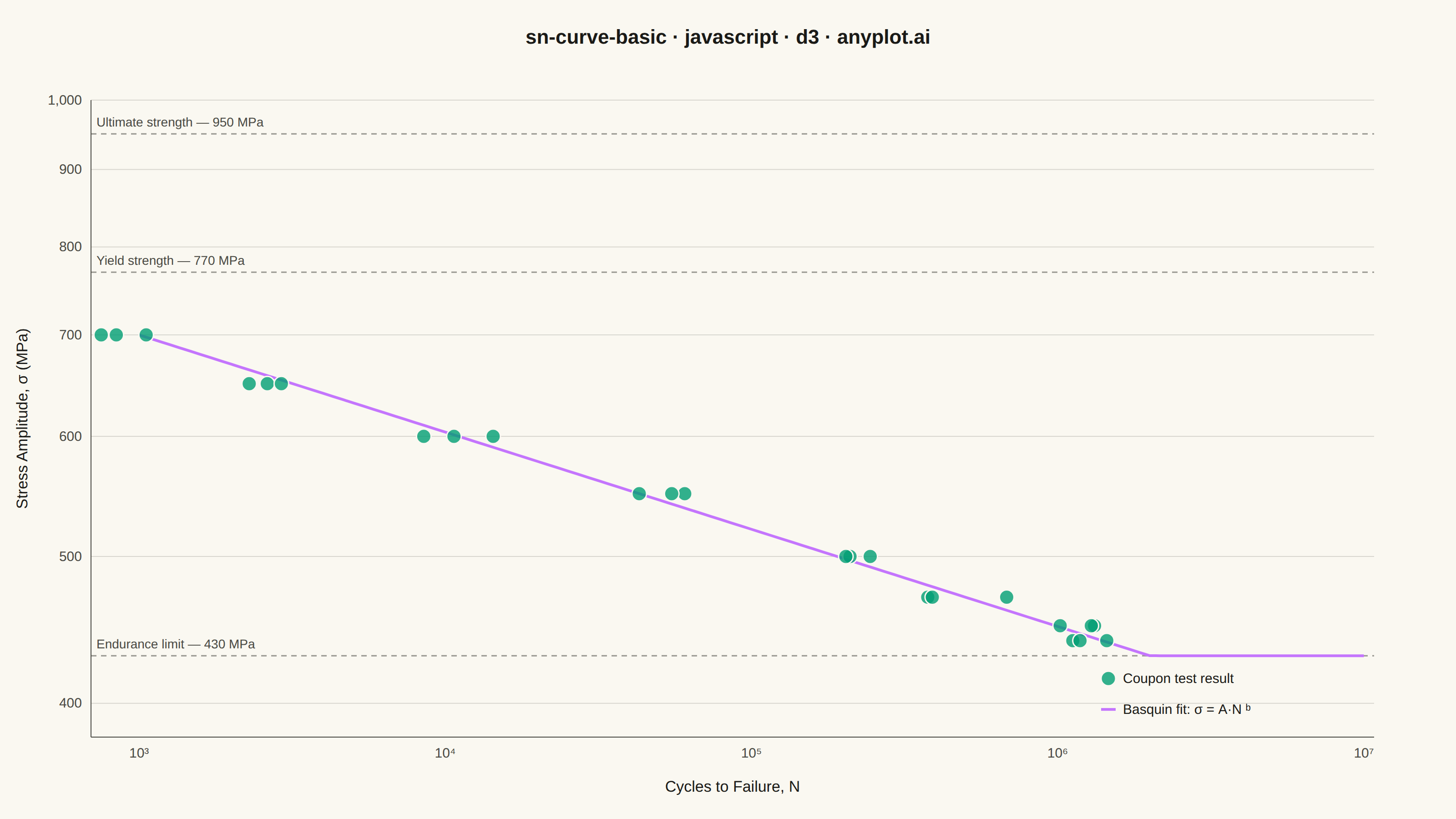
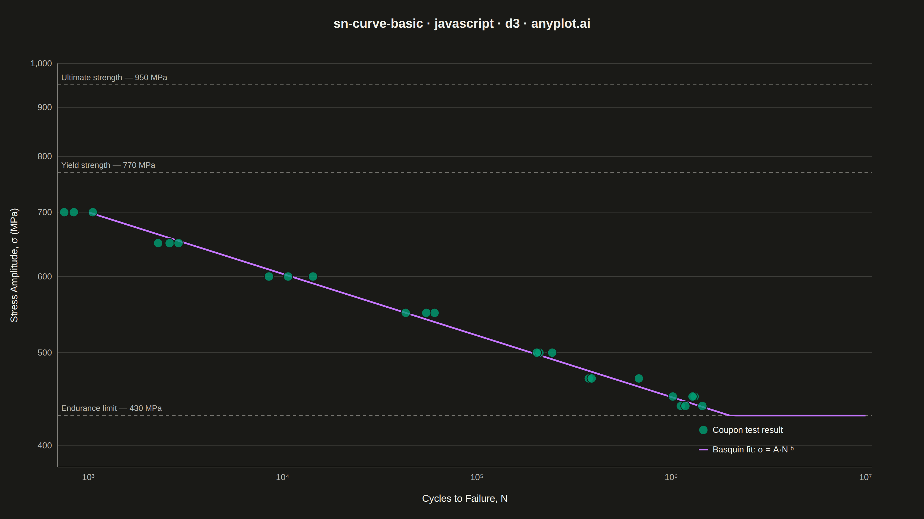
The same plot in 14 other libraries — JavaScript: Chart.js, Apache ECharts, Highcharts, MUI X Charts; Python: Altair, Bokeh, lets-plot, Matplotlib, Plotly, plotnine, Pygal, Seaborn; R: ggplot2; Julia: Makie.jl. Compare all 15 side by side: S-N Curve (Wöhler Curve) in Python, R, Julia and JavaScript.
An S-N curve (also known as a Wöhler curve) visualizes the relationship between alternating stress amplitude and the number of cycles to failure for a material under fatigue loading. Both axes typically use logarithmic scales, with stress on the y-axis and cycle count on the x-axis. This plot is fundamental for predicting material fatigue life and identifying key material properties such as ultimate strength, yield strength, and endurance limit.
// anyplot.ai
// sn-curve-basic: S-N Curve (Wöhler Curve)
// Library: d3 7.9.0 | JavaScript 22.23.2
// Quality: 90/100 | Created: 2026-09-02

const t = window.ANYPLOT_TOKENS;
const { width, height } = window.ANYPLOT_SIZE;
const margin = { top: 110, right: 90, bottom: 90, left: 100 };
const iw = width - margin.left - margin.right;
const ih = height - margin.top - margin.bottom;

// --- Data (in-memory, deterministic) ----------------------------------------
// AISI 4140 quenched-and-tempered steel: fully-reversed axial fatigue coupons.
function makeLcg(seed) {
  let s = seed;
  return () => {
    s = (s * 1664525 + 1013904223) % 4294967296;
    return s / 4294967296;
  };
}
const rand = makeLcg(42);

const ultimateStrength = 950; // MPa
const yieldStrength = 770; // MPa
const enduranceLimit = 430; // MPa
const transitionCycles = 2e6; // where the Basquin curve meets the endurance limit

// Basquin fit calibrated through (1e3 MPa @ 1e3 cycles) and (endurance @ transition)
const basquinN1 = 1e3;
const basquinS1 = 700;
const basquinB = Math.log(enduranceLimit / basquinS1) / Math.log(transitionCycles / basquinN1);
const basquinA = basquinS1 / Math.pow(basquinN1, basquinB);
const cyclesAtStress = (stress) => Math.pow(stress / basquinA, 1 / basquinB);
const stressAtCycles = (n) => (n <= transitionCycles ? basquinA * Math.pow(n, basquinB) : enduranceLimit);

const stressLevels = [700, 650, 600, 550, 500, 470, 450, 440];
const specimensPerLevel = 3;
const data = [];
for (const stress of stressLevels) {
  const baseCycles = cyclesAtStress(stress);
  for (let i = 0; i < specimensPerLevel; i++) {
    const jitterDecades = (rand() - 0.5) * 0.3; // scatter typical of coupon-to-coupon variation
    data.push({ stress, cycles: baseCycles * Math.pow(10, jitterDecades) });
  }
}

const fitMaxCycles = 1e7;
const fitSamples = d3.range(0, 121).map((i) => {
  const n = basquinN1 * Math.pow(fitMaxCycles / basquinN1, i / 120);
  return { cycles: n, stress: stressAtCycles(n) };
});

// --- Scales -------------------------------------------------------------------
// Derive the x domain from the actual jittered data (padded) instead of hardcoding
// [1e3, 1e7] — the 700 MPa level's base cycle count sits right at 1e3, and jitter
// can push some specimens below that fixed boundary.
const cycleExtent = d3.extent([...data.map((d) => d.cycles), basquinN1, fitMaxCycles]);
const domainPad = 1.08; // headroom so edge markers never clip against the axes
const x = d3
  .scaleLog()
  .domain([cycleExtent[0] / domainPad, cycleExtent[1] * domainPad])
  .range([0, iw]);
const y = d3.scaleLog().domain([380, 1000]).range([ih, 0]);

// --- SVG mount ------------------------------------------------------------
const svg = d3.select("#container").append("svg").attr("width", width).attr("height", height);
const g = svg.append("g").attr("transform", `translate(${margin.left},${margin.top})`);

// --- Grid (y-axis only, subtle) --------------------------------------------
g.append("g")
  .selectAll("line")
  .data(y.ticks(7))
  .join("line")
  .attr("x1", 0)
  .attr("x2", iw)
  .attr("y1", (d) => y(d))
  .attr("y2", (d) => y(d))
  .attr("stroke", t.grid)
  .attr("stroke-width", 1);

// --- Axes -----------------------------------------------------------------
const superscriptMap = { "-": "⁻", 0: "⁰", 1: "¹", 2: "²", 3: "³", 4: "⁴", 5: "⁵", 6: "⁶", 7: "⁷", 8: "⁸", 9: "⁹" };
const toSuperscript = (n) =>
  String(n)
    .split("")
    .map((c) => superscriptMap[c] ?? c)
    .join("");

const xTickValues = [1e3, 1e4, 1e5, 1e6, 1e7];
const xAxis = g
  .append("g")
  .attr("transform", `translate(0,${ih})`)
  .call(
    d3
      .axisBottom(x)
      .tickValues(xTickValues)
      .tickFormat((d) => `10${toSuperscript(Math.round(Math.log10(d)))}`)
      .tickSize(0)
      .tickPadding(12),
  );
xAxis.selectAll("text").attr("fill", t.inkSoft).style("font-size", "15px");
xAxis.select(".domain").attr("stroke", t.inkSoft);

const yAxis = g.append("g").call(
  d3
    .axisLeft(y)
    .ticks(7)
    .tickFormat((d) => d3.format(",")(d))
    .tickSize(0)
    .tickPadding(10),
);
yAxis.selectAll("text").attr("fill", t.inkSoft).style("font-size", "15px");
yAxis.select(".domain").attr("stroke", t.inkSoft);

// --- Reference lines: Ultimate Strength, Yield Strength, Endurance Limit ---
const references = [
  { label: "Ultimate strength", value: ultimateStrength },
  { label: "Yield strength", value: yieldStrength },
  { label: "Endurance limit", value: enduranceLimit },
];
const refLayer = g.append("g");
for (const ref of references) {
  const refY = y(ref.value);
  refLayer
    .append("line")
    .attr("x1", 0)
    .attr("x2", iw)
    .attr("y1", refY)
    .attr("y2", refY)
    .attr("stroke", t.inkSoft)
    .attr("stroke-width", 1.5)
    .attr("stroke-dasharray", "6 5")
    .attr("opacity", 0.55);
  refLayer
    .append("text")
    .attr("x", 6)
    .attr("y", refY - 8)
    .attr("fill", t.inkSoft)
    .style("font-size", "14px")
    .text(`${ref.label} — ${ref.value} MPa`);
}

// --- Basquin fit line --------------------------------------------------------
const line = d3
  .line()
  .x((d) => x(d.cycles))
  .y((d) => y(d.stress));
g.append("path")
  .datum(fitSamples)
  .attr("fill", "none")
  .attr("stroke", t.palette[1])
  .attr("stroke-width", 3)
  .attr("d", line);

// --- Data points ---------------------------------------------------------
g.selectAll("circle")
  .data(data)
  .join("circle")
  .attr("cx", (d) => x(d.cycles))
  .attr("cy", (d) => y(d.stress))
  .attr("r", 8)
  .attr("fill", t.palette[0])
  .attr("fill-opacity", 0.8)
  .attr("stroke", t.pageBg)
  .attr("stroke-width", 1.5);

// --- Legend ----------------------------------------------------------------
// Anchored below the endurance-limit line, which is always the lowest reference
// line and stays clear of the data cloud (no stress level plots below it) —
// unlike a fixed y, this never collides with a reference line or the scatter.
const legendY = y(enduranceLimit) + 25;
const legend = g.append("g").attr("transform", `translate(${iw - 300},${legendY})`);
legend
  .append("circle")
  .attr("cx", 8)
  .attr("cy", 0)
  .attr("r", 8)
  .attr("fill", t.palette[0])
  .attr("fill-opacity", 0.8)
  .attr("stroke", t.pageBg)
  .attr("stroke-width", 1.5);
legend.append("text").attr("x", 24).attr("y", 5).attr("fill", t.ink).style("font-size", "15px").text("Coupon test result");
legend
  .append("line")
  .attr("x1", 0)
  .attr("x2", 16)
  .attr("y1", 34)
  .attr("y2", 34)
  .attr("stroke", t.palette[1])
  .attr("stroke-width", 3);
legend
  .append("text")
  .attr("x", 24)
  .attr("y", 39)
  .attr("fill", t.ink)
  .style("font-size", "15px")
  .text("Basquin fit: σ = A·N ᵇ");

// --- Axis labels -------------------------------------------------------------
g.append("text")
  .attr("x", iw / 2)
  .attr("y", ih + 60)
  .attr("text-anchor", "middle")
  .attr("fill", t.ink)
  .style("font-size", "17px")
  .text("Cycles to Failure, N");

g.append("text")
  .attr("transform", "rotate(-90)")
  .attr("x", -ih / 2)
  .attr("y", -70)
  .attr("text-anchor", "middle")
  .attr("fill", t.ink)
  .style("font-size", "17px")
  .text("Stress Amplitude, σ (MPa)");

// --- Title -------------------------------------------------------------------
svg
  .append("text")
  .attr("x", width / 2)
  .attr("y", 48)
  .attr("text-anchor", "middle")
  .attr("fill", t.ink)
  .style("font-size", "22px")
  .style("font-weight", "600")
  .text("sn-curve-basic · javascript · d3 · anyplot.ai");
Runnable source as JSON, for any HTTP client: https://api.anyplot.ai/specs/sn-curve-basic/d3/code. Any spec id and library id listed in llms-full.txt fit the same URL shape; every URL below is complete and callable.
{
  "spec_id": "sn-curve-basic",
  "language": "javascript",
  "library": "d3",
  "page": "https://anyplot.ai/sn-curve-basic/javascript/d3",
  "hub": "https://anyplot.ai/sn-curve-basic",
  "code_json": "https://api.anyplot.ai/specs/sn-curve-basic/d3/code",
  "spec_json": "https://api.anyplot.ai/specs/sn-curve-basic",
  "render_light_png": "https://storage.googleapis.com/anyplot-images/plots/sn-curve-basic/javascript/d3/plot-light.png",
  "render_dark_png": "https://storage.googleapis.com/anyplot-images/plots/sn-curve-basic/javascript/d3/plot-dark.png",
  "interactive_light_html": "https://storage.googleapis.com/anyplot-images/plots/sn-curve-basic/javascript/d3/plot-light.html",
  "interactive_dark_html": "https://storage.googleapis.com/anyplot-images/plots/sn-curve-basic/javascript/d3/plot-dark.html",
  "quality_score": 90.0,
  "license": "MIT",
  "guide": "https://anyplot.ai/llms.txt"
}
Part of S-N Curve (Wöhler Curve) on anyplot.ai.