The same plot in 14 other libraries — JavaScript: Chart.js, D3.js, Highcharts, MUI X Charts; Python: Altair, Bokeh, lets-plot, Matplotlib, Plotly, plotnine, Pygal, Seaborn; R: ggplot2; Julia: Makie.jl. Compare all 15 side by side: S-N Curve (Wöhler Curve) in Python, R, Julia and JavaScript.
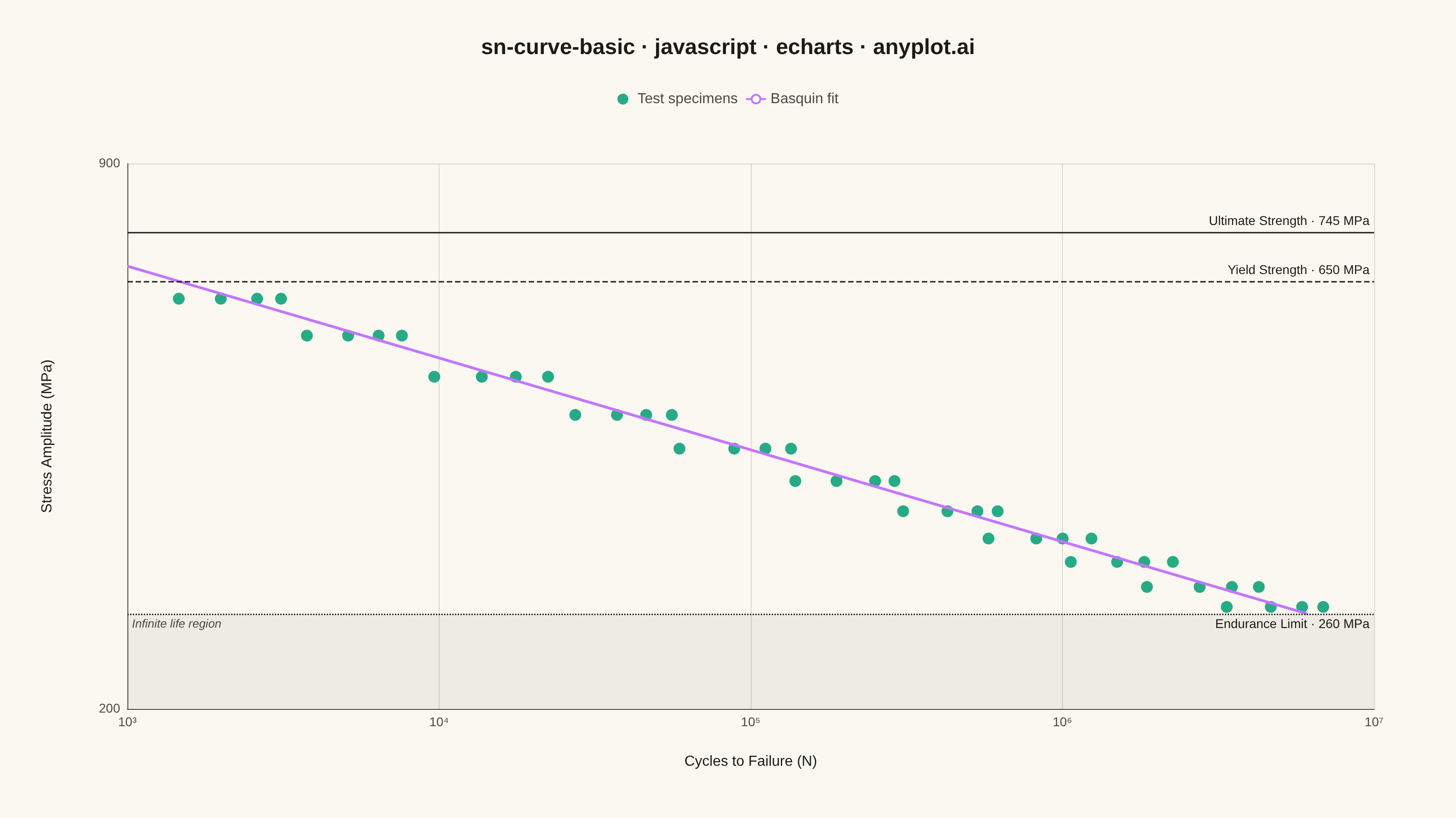
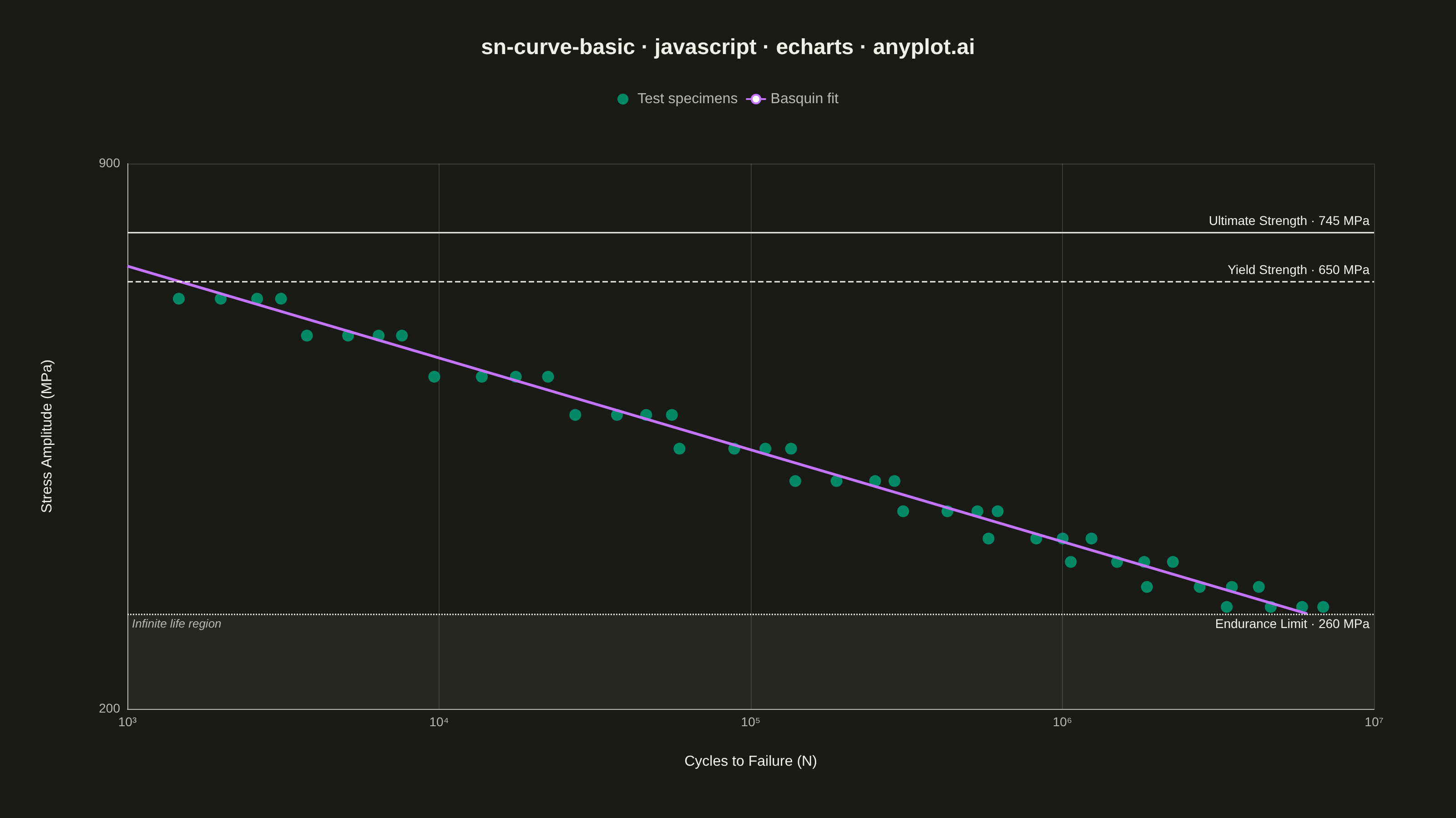
An S-N curve (also known as a Wöhler curve) visualizes the relationship between alternating stress amplitude and the number of cycles to failure for a material under fatigue loading. Both axes typically use logarithmic scales, with stress on the y-axis and cycle count on the x-axis. This plot is fundamental for predicting material fatigue life and identifying key material properties such as ultimate strength, yield strength, and endurance limit.
// anyplot.ai
// sn-curve-basic: S-N Curve (Wöhler Curve)
// Library: echarts 6.1.0 | JavaScript 22.23.2
// Quality: 89/100 | Created: 2026-09-02

const t = window.ANYPLOT_TOKENS;

// --- Data (in-memory, deterministic) ----------------------------------------
// Fatigue test data for a quenched-and-tempered 4340 steel coupon, fit with a
// Basquin power law: stress = fitA * cycles^fitB.
function lcg(seed) {
  let state = seed;
  return () => {
    state = (state * 1103515245 + 12345) % 2147483648;
    return state / 2147483648;
  };
}
const rand = lcg(42);

const ultimateStrength = 745; // MPa
const yieldStrength = 650; // MPa — ~0.87 of ultimate, typical for Q&T 4340 steel
const enduranceLimit = 260; // MPa
const fitA = 1450; // MPa — Basquin intercept
const fitB = -0.11; // Basquin exponent

// Nominal stress levels tested, multiple specimens per level (scatter in
// cycles-to-failure at fixed stress is the realistic fatigue-test outcome).
const stressLevels = [620, 560, 500, 450, 410, 375, 345, 320, 300, 280, 265];
const specimensPerLevel = 4;

const testPoints = [];
stressLevels.forEach((stress) => {
  const meanCycles = Math.pow(stress / fitA, 1 / fitB);
  for (let i = 0; i < specimensPerLevel; i++) {
    // Spread specimens deterministically around the mean so same-stress
    // clusters stay visually distinct instead of overlapping into one blob.
    const jitter = (i - (specimensPerLevel - 1) / 2) * 0.24;
    const scatterFactor = 1 + jitter + (rand() - 0.5) * 0.08;
    testPoints.push([meanCycles * scatterFactor, stress]);
  }
});

// Basquin fit curve, drawn from the low-cycle data down to the endurance limit.
const cyclesAtEndurance = Math.pow(enduranceLimit / fitA, 1 / fitB);
const logNStart = 3;
const logNEnd = Math.log10(cyclesAtEndurance);
const fitSteps = 60;
const fitCurve = [];
for (let i = 0; i <= fitSteps; i++) {
  const logN = logNStart + (i / fitSteps) * (logNEnd - logNStart);
  const cycles = Math.pow(10, logN);
  fitCurve.push([cycles, fitA * Math.pow(cycles, fitB)]);
}

// --- Helpers -----------------------------------------------------------------
const SUPERSCRIPTS = { 0: "⁰", 1: "¹", 2: "²", 3: "³", 4: "⁴", 5: "⁵", 6: "⁶", 7: "⁷", 8: "⁸", 9: "⁹" };
function formatDecadeTick(value) {
  const exponent = Math.log10(value);
  if (Math.abs(exponent - Math.round(exponent)) > 1e-6) return "";
  const digits = String(Math.round(exponent)).split("");
  return "10" + digits.map((d) => SUPERSCRIPTS[d] ?? d).join("");
}

// --- Init ---------------------------------------------------------------------
const chart = echarts.init(document.getElementById("container"));

// --- Option ---------------------------------------------------------------------
chart.setOption({
  animation: false,
  color: t.palette,
  backgroundColor: "transparent",
  title: {
    text: "sn-curve-basic · javascript · echarts · anyplot.ai",
    left: "center",
    top: 36,
    textStyle: { color: t.ink, fontSize: 24, fontWeight: 600 },
  },
  legend: {
    data: ["Test specimens", "Basquin fit"],
    top: 96,
    left: "center",
    itemWidth: 22,
    itemHeight: 12,
    textStyle: { color: t.inkSoft, fontSize: 16 },
  },
  tooltip: {
    trigger: "item",
    backgroundColor: t.elevatedBg,
    borderColor: t.grid,
    textStyle: { color: t.ink },
    valueFormatter: (value) => Math.round(value).toLocaleString(),
  },
  grid: { left: 140, right: 90, top: 180, bottom: 120 },
  xAxis: {
    type: "log",
    min: 1e3,
    max: 1e7,
    name: "Cycles to Failure (N)",
    nameLocation: "middle",
    nameGap: 50,
    nameTextStyle: { color: t.ink, fontSize: 16 },
    axisLabel: { color: t.inkSoft, fontSize: 14, formatter: formatDecadeTick },
    axisLine: { lineStyle: { color: t.inkSoft } },
    axisTick: { show: false },
    splitLine: { show: true, lineStyle: { color: t.grid } },
  },
  yAxis: {
    type: "log",
    min: 200,
    max: 900,
    name: "Stress Amplitude (MPa)",
    nameLocation: "middle",
    nameGap: 80,
    nameRotate: 90,
    nameTextStyle: { color: t.ink, fontSize: 16 },
    axisLabel: { color: t.inkSoft, fontSize: 14 },
    axisLine: { lineStyle: { color: t.inkSoft } },
    axisTick: { show: false },
    splitLine: { show: true, lineStyle: { color: t.grid } },
  },
  series: [
    {
      name: "Test specimens",
      type: "scatter",
      data: testPoints,
      symbolSize: 13,
      itemStyle: { color: t.palette[0], opacity: 0.85 },
    },
    {
      name: "Basquin fit",
      type: "line",
      data: fitCurve,
      showSymbol: false,
      lineStyle: { color: t.palette[1], width: 3 },
      itemStyle: { color: t.palette[1] },
      markArea: {
        silent: true,
        itemStyle: { color: t.ink, opacity: 0.06 },
        label: { show: true, position: "insideTopLeft", color: t.inkSoft, fontSize: 13, fontStyle: "italic" },
        data: [[{ yAxis: 200, name: "Infinite life region" }, { yAxis: enduranceLimit }]],
      },
      markLine: {
        silent: true,
        symbol: "none",
        label: { color: t.ink, fontSize: 14, position: "insideEndTop" },
        lineStyle: { color: t.ink, width: 1.5 },
        data: [
          {
            yAxis: ultimateStrength,
            lineStyle: { type: "solid" },
            label: { formatter: "Ultimate Strength · {c} MPa" },
          },
          {
            yAxis: yieldStrength,
            lineStyle: { type: "dashed" },
            label: { formatter: "Yield Strength · {c} MPa" },
          },
          {
            yAxis: enduranceLimit,
            lineStyle: { type: "dotted" },
            label: { formatter: "Endurance Limit · {c} MPa", position: "insideEndBottom" },
          },
        ],
      },
    },
  ],
});
Runnable source as JSON, for any HTTP client: https://api.anyplot.ai/specs/sn-curve-basic/echarts/code. Any spec id and library id listed in llms-full.txt fit the same URL shape; every URL below is complete and callable.
{
  "spec_id": "sn-curve-basic",
  "language": "javascript",
  "library": "echarts",
  "page": "https://anyplot.ai/sn-curve-basic/javascript/echarts",
  "hub": "https://anyplot.ai/sn-curve-basic",
  "code_json": "https://api.anyplot.ai/specs/sn-curve-basic/echarts/code",
  "spec_json": "https://api.anyplot.ai/specs/sn-curve-basic",
  "render_light_png": "https://storage.googleapis.com/anyplot-images/plots/sn-curve-basic/javascript/echarts/plot-light.png",
  "render_dark_png": "https://storage.googleapis.com/anyplot-images/plots/sn-curve-basic/javascript/echarts/plot-dark.png",
  "interactive_light_html": "https://storage.googleapis.com/anyplot-images/plots/sn-curve-basic/javascript/echarts/plot-light.html",
  "interactive_dark_html": "https://storage.googleapis.com/anyplot-images/plots/sn-curve-basic/javascript/echarts/plot-dark.html",
  "quality_score": 89.0,
  "license": "MIT",
  "guide": "https://anyplot.ai/llms.txt"
}
Part of S-N Curve (Wöhler Curve) on anyplot.ai.