The same plot in 14 other libraries — Python: Altair, Bokeh, lets-plot, Matplotlib, Plotly, plotnine, Pygal, Seaborn; Julia: Makie.jl; JavaScript: Chart.js, D3.js, Apache ECharts, Highcharts, MUI X Charts. Compare all 15 side by side: Wind Barb Plot for Meteorological Data in Python, R, Julia and JavaScript.
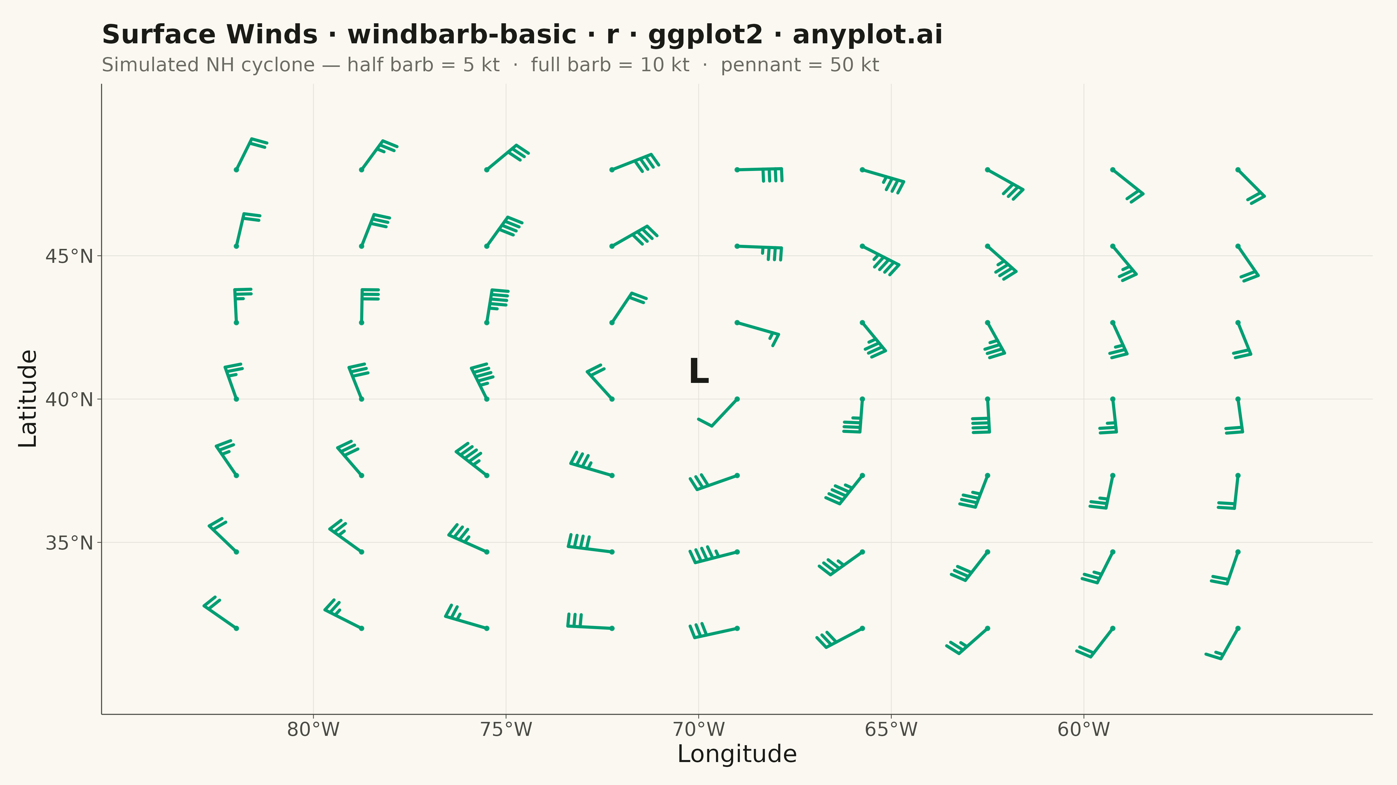
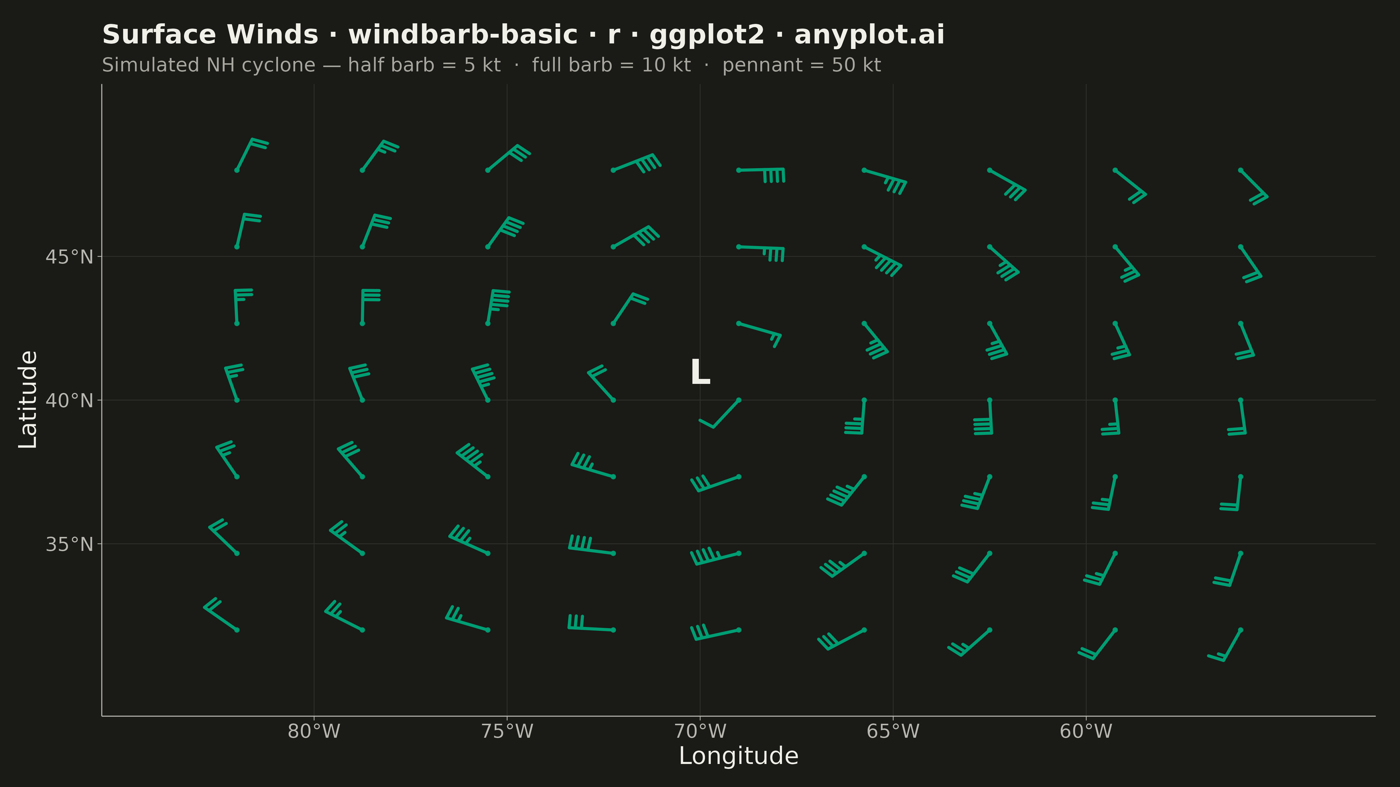
A wind barb plot displays wind speed and direction at specific locations using standard meteorological barb notation. Each barb consists of a staff pointing in the direction from which the wind blows, with short barbs (5 knots), long barbs (10 knots), and triangular pennants (50 knots) attached to indicate speed. This internationally recognized symbology enables rapid interpretation of wind patterns across weather maps and atmospheric data visualizations.
#' anyplot.ai
#' windbarb-basic: Wind Barb Plot for Meteorological Data
#' Library: ggplot2 3.5.1 | R 4.4.1
#' Quality: 86/100 | Created: 2026-05-19

library(ggplot2)
library(dplyr)
library(ragg)

set.seed(42)

# --- Theme tokens -------------------------------------------------------------
THEME       <- Sys.getenv("ANYPLOT_THEME", "light")
PAGE_BG     <- if (THEME == "light") "#FAF8F1" else "#1A1A17"
INK         <- if (THEME == "light") "#1A1A17" else "#F0EFE8"
INK_SOFT    <- if (THEME == "light") "#4A4A44" else "#B8B7B0"
INK_MUTED   <- if (THEME == "light") "#6B6A63" else "#A8A79F"
GRID_COLOR  <- if (THEME == "light") "#E4E2DB" else "#2F2F2C"
IMPRINT   <- c("#009E73", "#C475FD", "#4467A3", "#BD8233",
                 "#AE3030", "#2ABCCD", "#954477")
BARB_COLOR  <- IMPRINT[1]

# --- Wind field data ----------------------------------------------------------
# 9x7 grid of surface weather stations over eastern North America
# Simulates a Northern Hemisphere cyclone (counterclockwise circulation)
nx <- 9; ny <- 7
lons <- seq(-82, -56, length.out = nx)
lats <- seq(32, 48, length.out = ny)
stations <- expand.grid(lon = lons, lat = lats)

cx <- -70; cy <- 41             # low-pressure centre
dr_lon <- stations$lon - cx
dr_lat <- stations$lat - cy
r      <- sqrt(dr_lon^2 + dr_lat^2)

# Rankine vortex: speed rises to r_max then falls off
r_max   <- 6.0
max_spd <- 55                   # knots at peak radius
speed_kt <- ifelse(r < r_max,
                   max_spd * r / r_max,
                   max_spd * r_max / pmax(r, 0.01))

# CCW rotation (NH cyclone) with 15 % inward convergence
tan_lon  <- -dr_lat;  tan_lat <- dr_lon
tan_norm <- pmax(sqrt(tan_lon^2 + tan_lat^2), 0.01)
inward_lon <- -dr_lon / pmax(r, 0.01)
inward_lat <- -dr_lat / pmax(r, 0.01)
inflow  <- 0.15

stations$u <- ((tan_lon / tan_norm) * (1 - inflow) + inward_lon * inflow) * speed_kt
stations$v <- ((tan_lat / tan_norm) * (1 - inflow) + inward_lat * inflow) * speed_kt

# --- Barb geometry ------------------------------------------------------------
STAFF_LEN <- 1.15   # staff length in degrees
BARB_LEN  <- 0.42   # full barb feather length in degrees
BARB_SP   <- 0.16   # spacing between barbs along the staff

# Build segment list and pennant polygon list for one station.
# Standard meteorological barb convention (Northern Hemisphere):
#   staff  = points FROM which wind blows
#   barbs  = right of the staff when looking from base to tip
#   half barb = 5 kt, full barb = 10 kt, pennant (filled triangle) = 50 kt
make_barb_geometry <- function(x0, y0, u, v, staff_len, barb_len, barb_sp) {
  spd <- sqrt(u^2 + v^2)
  if (is.na(spd) || spd < 2.5) {
    return(list(segs = NULL, pens = NULL, calm = data.frame(x = x0, y = y0)))
  }

  ux <- -u / spd;  uy <- -v / spd   # staff unit vector (upwind direction)
  bx <-  uy;       by <- -ux        # barb unit vector (right of staff, NH)

  segs_list <- list()
  pen_list  <- list()

  # Staff
  segs_list[[1]] <- data.frame(
    x    = x0,                   y    = y0,
    xend = x0 + staff_len * ux,  yend = y0 + staff_len * uy
  )

  # Decompose rounded speed into barb counts
  spd_r <- round(spd / 5) * 5
  n50   <- spd_r %/% 50;  rem <- spd_r - n50 * 50
  n10   <- rem   %/% 10;  rem <- rem   - n10 * 10
  n5    <- rem   %/% 5

  pos <- staff_len   # current position along staff from base, start at tip

  # Pennants (50 kt each) — filled triangles placed first from the tip
  for (i in seq_len(n50)) {
    tx  <- x0 + pos * ux;                ty  <- y0 + pos * uy
    bx2 <- x0 + (pos - barb_sp) * ux;   by2 <- y0 + (pos - barb_sp) * uy
    px  <- bx2 + barb_len * bx;         py  <- by2 + barb_len * by
    pen_list[[length(pen_list) + 1]] <- data.frame(
      x      = c(tx, bx2, px),
      y      = c(ty, by2, py),
      pen_id = paste0(round(x0, 3), "_", round(y0, 3), "_p", i)
    )
    pos <- pos - barb_sp
  }

  # Full barbs (10 kt each)
  for (i in seq_len(n10)) {
    ax <- x0 + pos * ux;  ay <- y0 + pos * uy
    segs_list[[length(segs_list) + 1]] <- data.frame(
      x    = ax,  y    = ay,
      xend = ax + barb_len * bx,  yend = ay + barb_len * by
    )
    pos <- pos - barb_sp
  }

  # Half barbs (5 kt each)
  for (i in seq_len(n5)) {
    ax <- x0 + pos * ux;  ay <- y0 + pos * uy
    segs_list[[length(segs_list) + 1]] <- data.frame(
      x    = ax,  y    = ay,
      xend = ax + 0.5 * barb_len * bx,  yend = ay + 0.5 * barb_len * by
    )
    pos <- pos - barb_sp
  }

  list(
    segs = do.call(rbind, segs_list),
    pens = if (length(pen_list) > 0) do.call(rbind, pen_list) else NULL,
    calm = NULL
  )
}

# Collect geometry for all stations
geom_list <- lapply(seq_len(nrow(stations)), function(i) {
  make_barb_geometry(stations$lon[i], stations$lat[i],
                     stations$u[i], stations$v[i],
                     STAFF_LEN, BARB_LEN, BARB_SP)
})

barb_segs <- do.call(rbind, lapply(geom_list, function(g) g$segs))
pennants  <- do.call(rbind, lapply(geom_list, function(g) g$pens))
calm_pts  <- do.call(rbind, lapply(geom_list, function(g) g$calm))
station_pts <- data.frame(x = stations$lon, y = stations$lat)

# --- Plot --------------------------------------------------------------------
p <- ggplot() +
  geom_point(data = station_pts, aes(x = x, y = y),
             color = BARB_COLOR, size = 1.4, alpha = 0.9) +
  geom_segment(data = barb_segs,
               aes(x = x, y = y, xend = xend, yend = yend),
               color = BARB_COLOR, linewidth = 1.2, lineend = "round")

if (!is.null(pennants) && nrow(pennants) > 0) {
  p <- p + geom_polygon(data = pennants, aes(x = x, y = y, group = pen_id),
                         fill = BARB_COLOR, color = NA)
}

if (!is.null(calm_pts) && nrow(calm_pts) > 0) {
  p <- p + geom_point(data = calm_pts, aes(x = x, y = y),
                       shape = 1, color = BARB_COLOR, size = 5, stroke = 1.5)
}

p <- p +
  annotate("text", x = cx, y = cy, label = "L",
           color = INK, size = 10, fontface = "bold") +
  scale_x_continuous(breaks = seq(-80, -60, by = 5),
                     labels = function(x) paste0(abs(x), "°W")) +
  scale_y_continuous(breaks = seq(35, 45, by = 5),
                     labels = function(y) paste0(y, "°N")) +
  coord_cartesian(xlim = c(-84, -54), ylim = c(30, 50)) +
  labs(
    title    = paste0("Surface Winds · windbarb-basic · r · ggplot2 · anyplot.ai"),
    subtitle = "Simulated NH cyclone — half barb = 5 kt  ·  full barb = 10 kt  ·  pennant = 50 kt",
    x        = "Longitude",
    y        = "Latitude"
  ) +
  theme_minimal(base_size = 14) +
  theme(
    plot.background  = element_rect(fill = PAGE_BG, color = PAGE_BG),
    panel.background = element_rect(fill = PAGE_BG, color = NA),
    panel.grid.major = element_line(color = GRID_COLOR, linewidth = 0.3),
    panel.grid.minor = element_blank(),
    panel.border     = element_blank(),
    axis.line        = element_line(color = INK_SOFT, linewidth = 0.4),
    axis.ticks       = element_line(color = INK_SOFT, linewidth = 0.3),
    axis.title       = element_text(color = INK,       size = 20),
    axis.text        = element_text(color = INK_SOFT,  size = 16),
    plot.title       = element_text(color = INK,       size = 22, face = "bold"),
    plot.subtitle    = element_text(color = INK_MUTED, size = 16),
    plot.margin      = margin(t = 20, r = 20, b = 15, l = 15)
  )

# --- Save --------------------------------------------------------------------
ggsave(
  filename = sprintf("plot-%s.png", THEME),
  plot     = p,
  device   = ragg::agg_png,
  width    = 16,
  height   = 9,
  units    = "in",
  dpi      = 300
)
Runnable source as JSON, for any HTTP client: https://api.anyplot.ai/specs/windbarb-basic/ggplot2/code. Any spec id and library id listed in llms-full.txt fit the same URL shape; every URL below is complete and callable.
{
  "spec_id": "windbarb-basic",
  "language": "r",
  "library": "ggplot2",
  "page": "https://anyplot.ai/windbarb-basic/r/ggplot2",
  "hub": "https://anyplot.ai/windbarb-basic",
  "code_json": "https://api.anyplot.ai/specs/windbarb-basic/ggplot2/code",
  "spec_json": "https://api.anyplot.ai/specs/windbarb-basic",
  "render_light_png": "https://storage.googleapis.com/anyplot-images/plots/windbarb-basic/r/ggplot2/plot-light.png",
  "render_dark_png": "https://storage.googleapis.com/anyplot-images/plots/windbarb-basic/r/ggplot2/plot-dark.png",
  "quality_score": 86.0,
  "license": "MIT",
  "guide": "https://anyplot.ai/llms.txt"
}
Part of Wind Barb Plot for Meteorological Data on anyplot.ai.