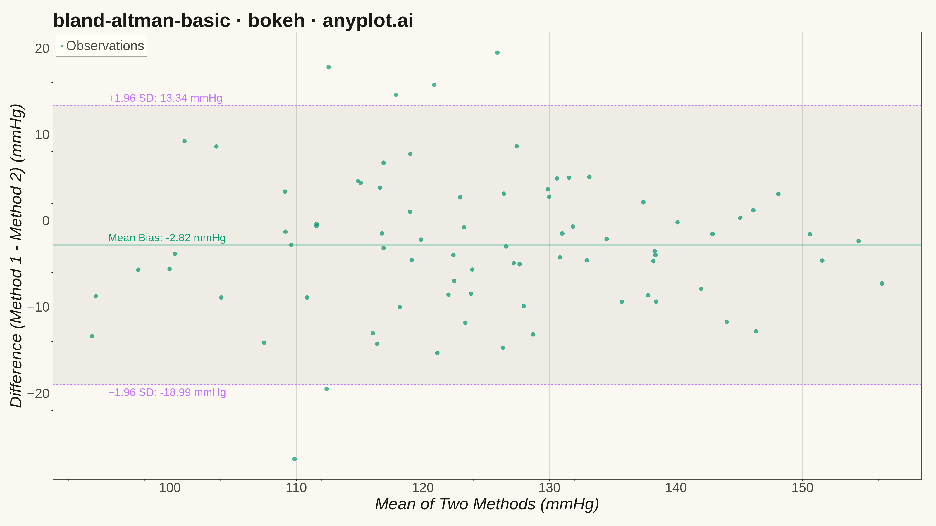
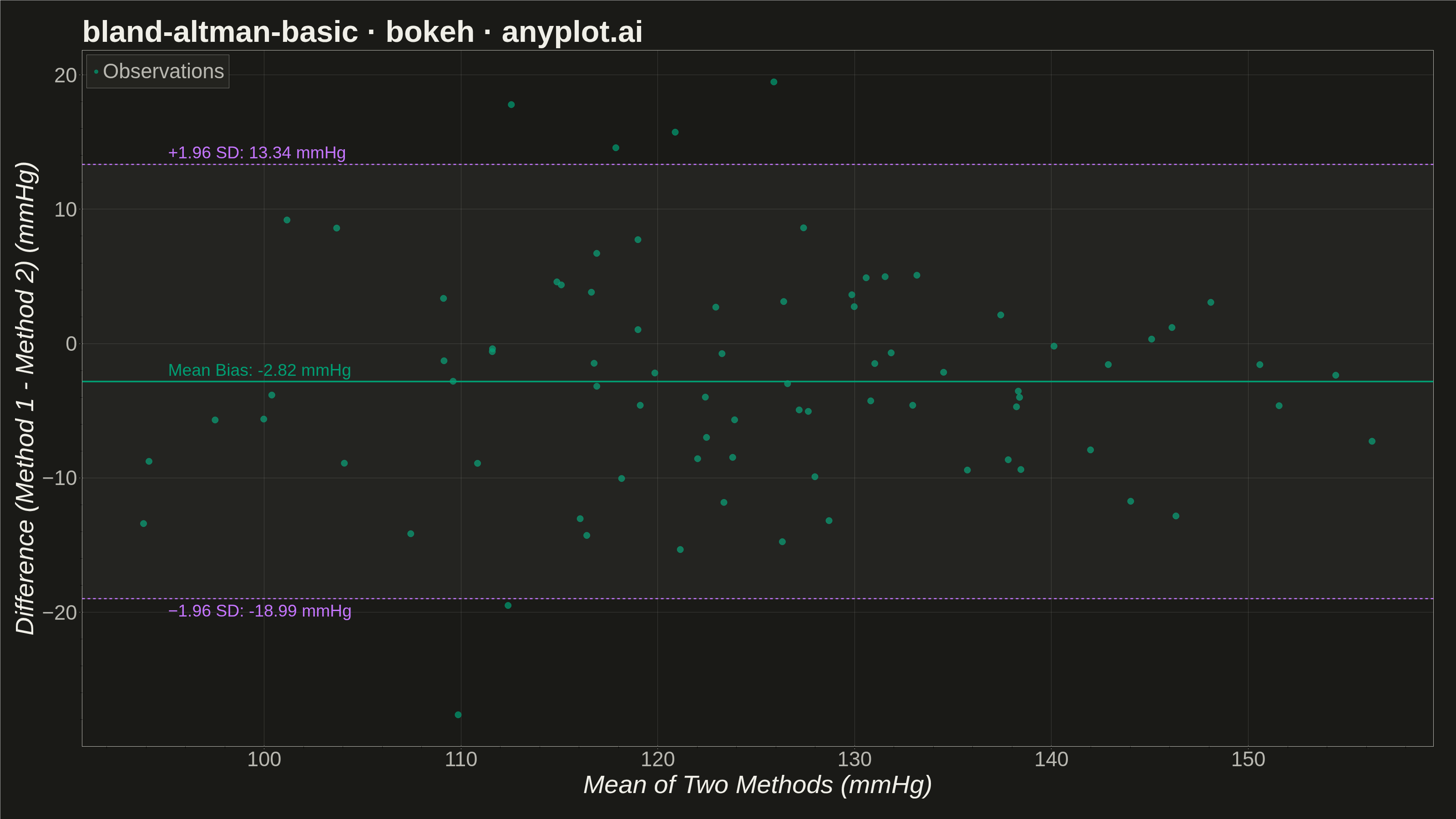
A Bland-Altman plot (also known as a difference plot or Tukey mean-difference plot) visualizes the agreement between two measurement methods by plotting the difference against the average of paired observations. It displays the mean difference (bias) as a horizontal line and limits of agreement (mean ± 1.96 SD) to assess whether the methods are interchangeable within acceptable tolerances.
""" anyplot.ai
bland-altman-basic: Bland-Altman Agreement Plot
Library: bokeh 3.9.2 | Python 3.13.14
Quality: 90/100 | Updated: 2026-08-11
"""

import os
import time
from pathlib import Path

import numpy as np
from bokeh.io import output_file, save
from bokeh.models import BoxAnnotation, ColumnDataSource, HoverTool, Label, Span
from bokeh.plotting import figure
from selenium import webdriver
from selenium.webdriver.chrome.options import Options


THEME = os.getenv("ANYPLOT_THEME", "light")
PAGE_BG = "#FAF8F1" if THEME == "light" else "#1A1A17"
ELEVATED_BG = "#FFFDF6" if THEME == "light" else "#242420"
INK = "#1A1A17" if THEME == "light" else "#F0EFE8"
INK_SOFT = "#4A4A44" if THEME == "light" else "#B8B7B0"

BRAND = "#009E73"
ACCENT = "#C475FD"

np.random.seed(42)
n = 80

true_bp = np.random.normal(125, 15, n)
method1 = true_bp + np.random.normal(0, 5, n)
method2 = true_bp + np.random.normal(2, 6, n)

mean_values = (method1 + method2) / 2
diff_values = method1 - method2
mean_diff = np.mean(diff_values)
std_diff = np.std(diff_values, ddof=1)
upper_loa = mean_diff + 1.96 * std_diff
lower_loa = mean_diff - 1.96 * std_diff

source = ColumnDataSource(data={"mean": mean_values, "diff": diff_values})

# `width` / `height` are the TOTAL canvas; axis labels at the 36-42pt
# native-pixel sizes need explicit `min_border_*` reservations or they get
# clipped at the edges of the rendered PNG.
p = figure(
    width=3200,
    height=1800,
    title="bland-altman-basic · python · bokeh · anyplot.ai",
    x_axis_label="Mean of Two Methods (mmHg)",
    y_axis_label="Difference (Method 1 - Method 2) (mmHg)",
    toolbar_location=None,
    min_border_bottom=160,
    min_border_left=180,
    min_border_top=110,
    min_border_right=50,
)

# Subtle shaded band for the limits-of-agreement zone (design refinement:
# gives the +-1.96 SD region a visual footprint without competing with data).
agreement_zone = BoxAnnotation(bottom=lower_loa, top=upper_loa, fill_color=INK, fill_alpha=0.05)
p.add_layout(agreement_zone)

scatter_renderer = p.scatter(
    x="mean",
    y="diff",
    source=source,
    size=14,
    color=BRAND,
    alpha=0.7,
    line_color=PAGE_BG,
    line_width=1,
    legend_label="Observations",
)
p.add_tools(
    HoverTool(tooltips=[("Mean", "@mean{0.2f} mmHg"), ("Difference", "@diff{0.2f} mmHg")], renderers=[scatter_renderer])
)

mean_line = Span(location=mean_diff, dimension="width", line_color=BRAND, line_width=3.5, line_dash="solid")
p.add_layout(mean_line)

upper_line = Span(location=upper_loa, dimension="width", line_color=ACCENT, line_width=2.5, line_dash="dashed")
p.add_layout(upper_line)

lower_line = Span(location=lower_loa, dimension="width", line_color=ACCENT, line_width=2.5, line_dash="dashed")
p.add_layout(lower_line)

x_min = np.min(mean_values)
x_label_pos = x_min + (np.max(mean_values) - x_min) * 0.02

mean_label = Label(
    x=x_label_pos,
    y=mean_diff,
    text=f"Mean Bias: {mean_diff:.2f} mmHg",
    text_font_size="28pt",
    text_color=BRAND,
    text_baseline="bottom",
    y_offset=5,
)
p.add_layout(mean_label)

upper_label = Label(
    x=x_label_pos,
    y=upper_loa,
    text=f"+1.96 SD: {upper_loa:.2f} mmHg",
    text_font_size="28pt",
    text_color=ACCENT,
    text_baseline="bottom",
    y_offset=5,
)
p.add_layout(upper_label)

lower_label = Label(
    x=x_label_pos,
    y=lower_loa,
    text=f"−1.96 SD: {lower_loa:.2f} mmHg",
    text_font_size="28pt",
    text_color=ACCENT,
    text_baseline="top",
    y_offset=-5,
)
p.add_layout(lower_label)

p.title.text_font_size = "50pt"
p.title.text_color = INK
p.xaxis.axis_label_text_font_size = "42pt"
p.yaxis.axis_label_text_font_size = "42pt"
p.xaxis.axis_label_text_color = INK
p.yaxis.axis_label_text_color = INK
p.xaxis.major_label_text_font_size = "34pt"
p.yaxis.major_label_text_font_size = "34pt"
p.xaxis.major_label_text_color = INK_SOFT
p.yaxis.major_label_text_color = INK_SOFT

p.xaxis.axis_line_color = INK_SOFT
p.yaxis.axis_line_color = INK_SOFT
p.xaxis.major_tick_line_color = INK_SOFT
p.yaxis.major_tick_line_color = INK_SOFT

p.xgrid.grid_line_color = INK
p.ygrid.grid_line_color = INK
p.xgrid.grid_line_alpha = 0.15
p.ygrid.grid_line_alpha = 0.15

p.background_fill_color = PAGE_BG
p.border_fill_color = PAGE_BG
# No-frame treatment: bokeh's `outline_line_color` draws a single rectangle
# around the whole plot area (no per-side spine control like matplotlib), so
# a full box is the only "outline" option — skip it in favor of the axis
# lines alone for a cleaner, less boxed-in look.
p.outline_line_color = None

if p.legend:
    p.legend.label_text_font_size = "34pt"
    p.legend.label_text_color = INK_SOFT
    p.legend.location = "top_left"
    p.legend.background_fill_color = ELEVATED_BG
    p.legend.border_line_color = INK_SOFT

output_file(f"plot-{THEME}.html")
save(p)

# IMPORTANT: W,H must match the figure's width/height above, otherwise the
# bokeh canvas paints into the upper-left corner with white space around it.
W, H = 3200, 1800
opts = Options()
for arg in (
    "--headless=new",
    "--no-sandbox",
    "--disable-dev-shm-usage",
    "--disable-gpu",
    f"--window-size={W},{H}",
    "--hide-scrollbars",
):
    opts.add_argument(arg)
driver = webdriver.Chrome(options=opts)
driver.set_window_size(W, H)
driver.get(f"file://{Path(f'plot-{THEME}.html').resolve()}")
# IMPORTANT: headless Chrome's --window-size sets the OUTER window, which still
# reserves a phantom title-bar height even headless — innerHeight (and thus the
# screenshot) comes out short of H. Pin the viewport exactly via CDP.
driver.execute_cdp_cmd(
    "Emulation.setDeviceMetricsOverride", {"width": W, "height": H, "deviceScaleFactor": 1, "mobile": False}
)
time.sleep(3)
driver.save_screenshot(f"plot-{THEME}.png")
driver.quit()
Runnable source as JSON, for any HTTP client: https://api.anyplot.ai/specs/bland-altman-basic/bokeh/code. Any spec id and library id listed in llms-full.txt fit the same URL shape; every URL below is complete and callable.
{
  "spec_id": "bland-altman-basic",
  "language": "python",
  "library": "bokeh",
  "page": "https://anyplot.ai/bland-altman-basic/python/bokeh",
  "hub": "https://anyplot.ai/bland-altman-basic",
  "code_json": "https://api.anyplot.ai/specs/bland-altman-basic/bokeh/code",
  "spec_json": "https://api.anyplot.ai/specs/bland-altman-basic",
  "render_light_png": "https://storage.googleapis.com/anyplot-images/plots/bland-altman-basic/python/bokeh/plot-light.png",
  "render_dark_png": "https://storage.googleapis.com/anyplot-images/plots/bland-altman-basic/python/bokeh/plot-dark.png",
  "interactive_light_html": "https://storage.googleapis.com/anyplot-images/plots/bland-altman-basic/python/bokeh/plot-light.html",
  "interactive_dark_html": "https://storage.googleapis.com/anyplot-images/plots/bland-altman-basic/python/bokeh/plot-dark.html",
  "quality_score": 90.0,
  "license": "MIT",
  "guide": "https://anyplot.ai/llms.txt"
}
Part of Bland-Altman Agreement Plot on anyplot.ai.