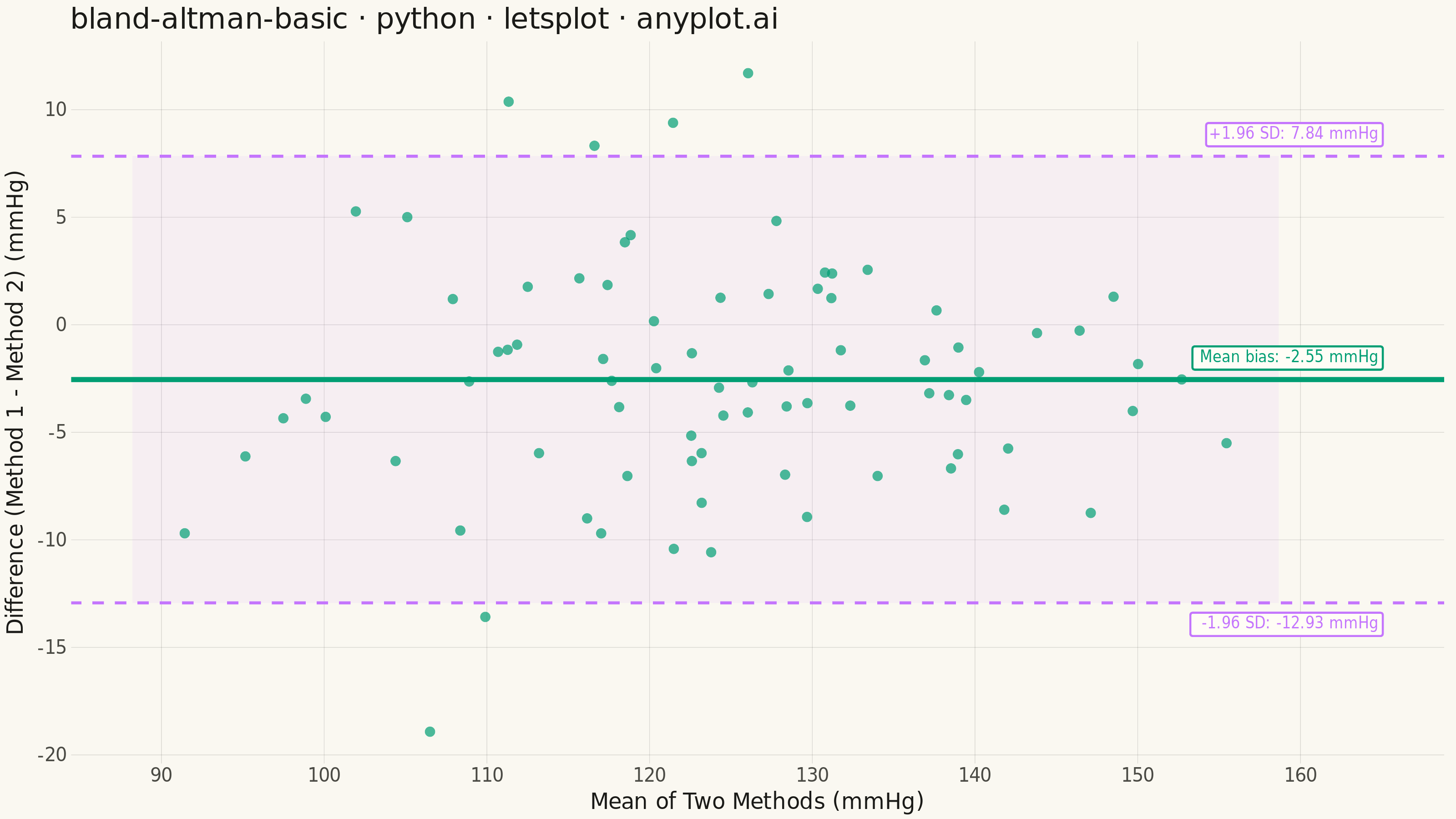
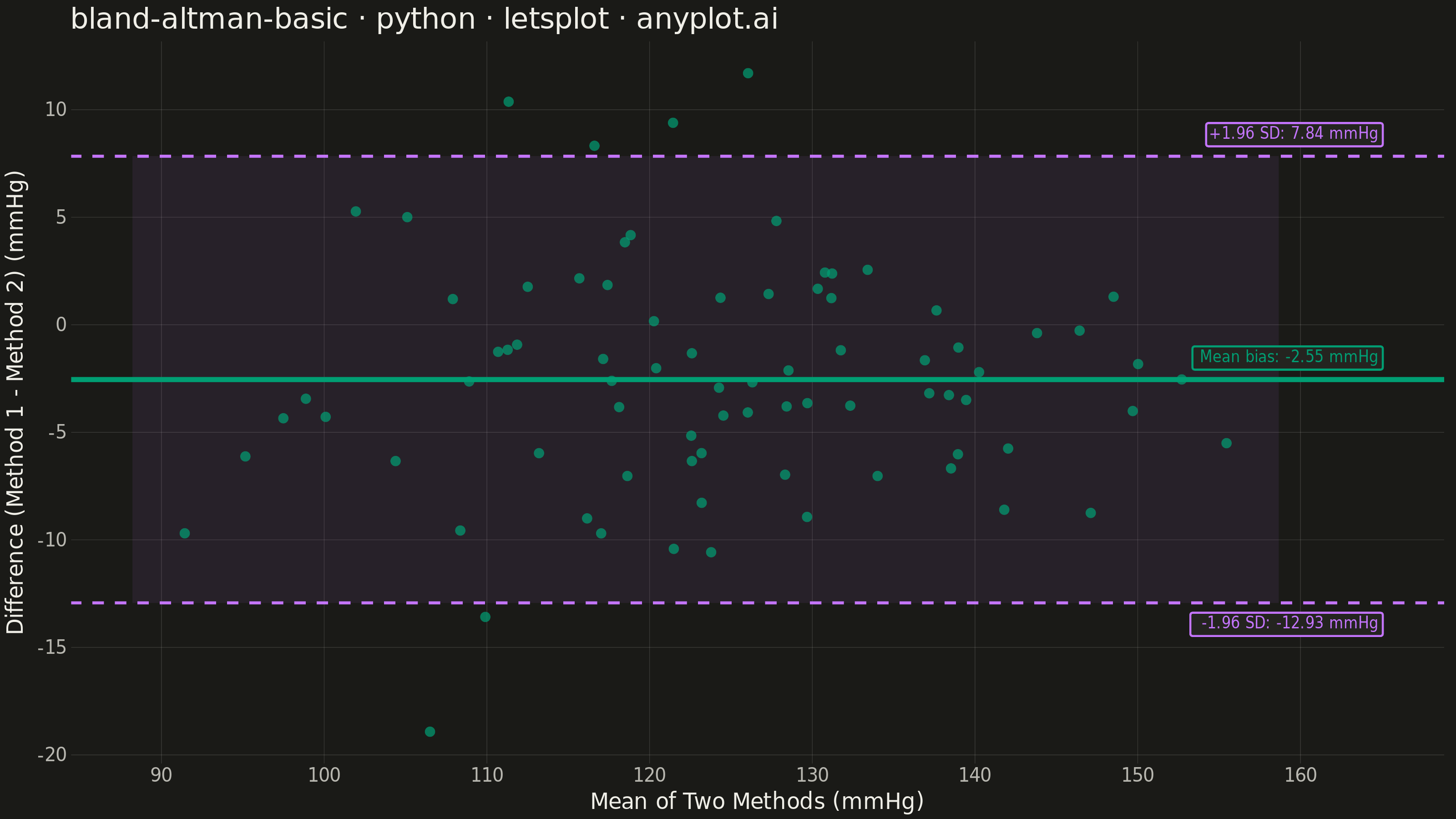
A Bland-Altman plot (also known as a difference plot or Tukey mean-difference plot) visualizes the agreement between two measurement methods by plotting the difference against the average of paired observations. It displays the mean difference (bias) as a horizontal line and limits of agreement (mean ± 1.96 SD) to assess whether the methods are interchangeable within acceptable tolerances.
""" anyplot.ai
bland-altman-basic: Bland-Altman Agreement Plot
Library: letsplot 4.11.0 | Python 3.13.14
Quality: 92/100 | Updated: 2026-08-11
"""

import os

import numpy as np
import pandas as pd
from lets_plot import (
    LetsPlot,
    aes,
    element_blank,
    element_line,
    element_rect,
    element_text,
    geom_hline,
    geom_label,
    geom_point,
    geom_rect,
    ggplot,
    ggsave,
    ggsize,
    labs,
    layer_tooltips,
    theme,
    theme_minimal,
)


LetsPlot.setup_html()

# Theme tokens
THEME = os.getenv("ANYPLOT_THEME", "light")
PAGE_BG = "#FAF8F1" if THEME == "light" else "#1A1A17"
ELEVATED_BG = "#FFFDF6" if THEME == "light" else "#242420"
INK = "#1A1A17" if THEME == "light" else "#F0EFE8"
INK_SOFT = "#4A4A44" if THEME == "light" else "#B8B7B0"
GRID_COLOR = "rgba(26,26,23,0.15)" if THEME == "light" else "rgba(240,239,232,0.15)"

# Imprint palette
BRAND = "#009E73"  # Position 1 - first categorical series
SECONDARY = "#C475FD"  # Position 2 - limits of agreement

# Data: Simulated blood pressure readings from two sphygmomanometers
np.random.seed(42)
n = 80

# True systolic BP values (realistic range: 100-160 mmHg)
true_bp = np.random.normal(125, 15, n)

# Method 1: Reference standard (small measurement error)
method1 = true_bp + np.random.normal(0, 3, n)

# Method 2: New device (slight positive bias + slightly larger error)
method2 = true_bp + np.random.normal(2, 4, n)

# Bland-Altman calculations
mean_values = (method1 + method2) / 2
diff_values = method1 - method2

mean_diff = np.mean(diff_values)
std_diff = np.std(diff_values, ddof=1)
upper_loa = mean_diff + 1.96 * std_diff
lower_loa = mean_diff - 1.96 * std_diff

# Point-level data - also drives the interactive hover tooltips
df = pd.DataFrame({"method1": method1, "method2": method2, "mean": mean_values, "diff": diff_values})

# Agreement band: shaded rectangle spanning the limits of agreement
x_pad = (df["mean"].max() - df["mean"].min()) * 0.05
band_df = pd.DataFrame(
    {"xmin": [df["mean"].min() - x_pad], "xmax": [df["mean"].max() + x_pad], "ymin": [lower_loa], "ymax": [upper_loa]}
)

# Annotation labels, right-aligned with extra headroom past the data range so the
# label never sits on top of whichever point happens to be rightmost
annot_x = df["mean"].max() + x_pad * 3
y_offset = 1.0
annot_df = pd.DataFrame(
    {
        "x": [annot_x, annot_x, annot_x],
        "y": [mean_diff + y_offset, upper_loa + y_offset, lower_loa - y_offset],
        "label": [
            f"Mean bias: {mean_diff:.2f} mmHg",
            f"+1.96 SD: {upper_loa:.2f} mmHg",
            f"-1.96 SD: {lower_loa:.2f} mmHg",
        ],
        "line_type": ["bias", "loa", "loa"],
    }
)

# Build plot with theme-adaptive styling
plot = (
    ggplot()
    + geom_rect(
        aes(xmin="xmin", xmax="xmax", ymin="ymin", ymax="ymax"), data=band_df, fill=SECONDARY, alpha=0.08, size=0
    )
    + geom_point(
        aes(x="mean", y="diff"),
        data=df,
        color=BRAND,
        size=2.5,
        alpha=0.7,
        stroke=0.4,
        tooltips=layer_tooltips()
        .line("Method 1|@method1")
        .line("Method 2|@method2")
        .line("Mean|@mean")
        .line("Difference|@diff"),
    )
    + geom_hline(yintercept=mean_diff, color=BRAND, size=1.2)
    + geom_hline(yintercept=upper_loa, color=SECONDARY, size=0.7, linetype="dashed")
    + geom_hline(yintercept=lower_loa, color=SECONDARY, size=0.7, linetype="dashed")
    + geom_label(
        aes(x="x", y="y", label="label"),
        data=annot_df[annot_df["line_type"] == "bias"],
        size=4,
        color=BRAND,
        fill=ELEVATED_BG,
        hjust=1,
        label_padding=0.3,
        label_r=0.1,
    )
    + geom_label(
        aes(x="x", y="y", label="label"),
        data=annot_df[annot_df["line_type"] == "loa"],
        size=4,
        color=SECONDARY,
        fill=ELEVATED_BG,
        hjust=1,
        label_padding=0.3,
        label_r=0.1,
    )
    + labs(
        x="Mean of Two Methods (mmHg)",
        y="Difference (Method 1 - Method 2) (mmHg)",
        title="bland-altman-basic · python · letsplot · anyplot.ai",
    )
    + ggsize(800, 450)
    + theme_minimal()
    + theme(
        plot_background=element_rect(fill=PAGE_BG, color=PAGE_BG),
        panel_background=element_rect(fill=PAGE_BG, color=PAGE_BG),
        panel_grid_major=element_line(color=GRID_COLOR, size=0.3, linetype="solid"),
        panel_grid_minor=element_blank(),
        plot_title=element_text(size=16, color=INK),
        axis_title=element_text(size=12, color=INK),
        axis_text=element_text(size=10, color=INK_SOFT),
        axis_line=element_line(color=INK_SOFT, size=0.5),
    )
)

# Save PNG and HTML with theme-suffixed filenames
ggsave(plot, f"plot-{THEME}.png", scale=4, path=".")
ggsave(plot, f"plot-{THEME}.html", path=".")
Runnable source as JSON, for any HTTP client: https://api.anyplot.ai/specs/bland-altman-basic/letsplot/code. Any spec id and library id listed in llms-full.txt fit the same URL shape; every URL below is complete and callable.
{
  "spec_id": "bland-altman-basic",
  "language": "python",
  "library": "letsplot",
  "page": "https://anyplot.ai/bland-altman-basic/python/letsplot",
  "hub": "https://anyplot.ai/bland-altman-basic",
  "code_json": "https://api.anyplot.ai/specs/bland-altman-basic/letsplot/code",
  "spec_json": "https://api.anyplot.ai/specs/bland-altman-basic",
  "render_light_png": "https://storage.googleapis.com/anyplot-images/plots/bland-altman-basic/python/letsplot/plot-light.png",
  "render_dark_png": "https://storage.googleapis.com/anyplot-images/plots/bland-altman-basic/python/letsplot/plot-dark.png",
  "interactive_light_html": "https://storage.googleapis.com/anyplot-images/plots/bland-altman-basic/python/letsplot/plot-light.html",
  "interactive_dark_html": "https://storage.googleapis.com/anyplot-images/plots/bland-altman-basic/python/letsplot/plot-dark.html",
  "quality_score": 92.0,
  "license": "MIT",
  "guide": "https://anyplot.ai/llms.txt"
}
Part of Bland-Altman Agreement Plot on anyplot.ai.