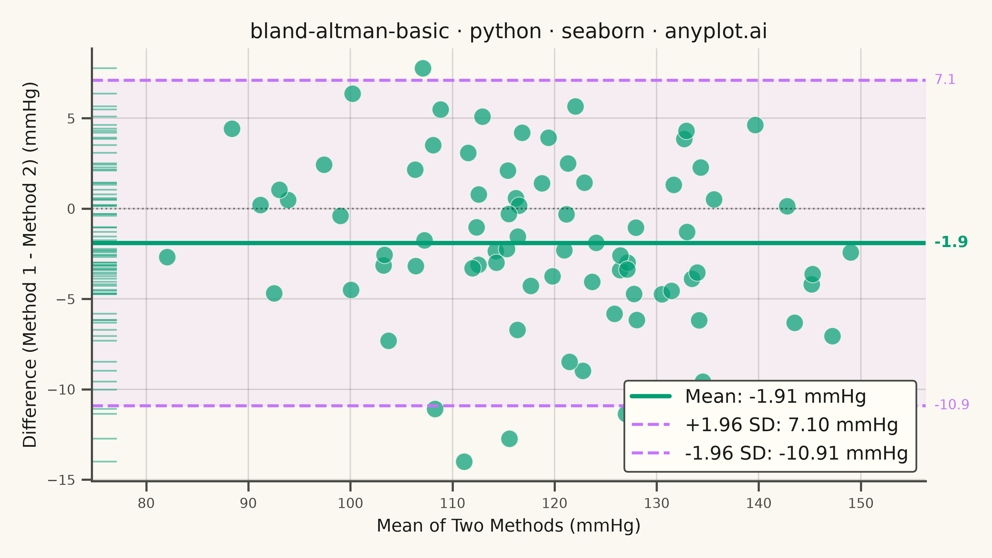
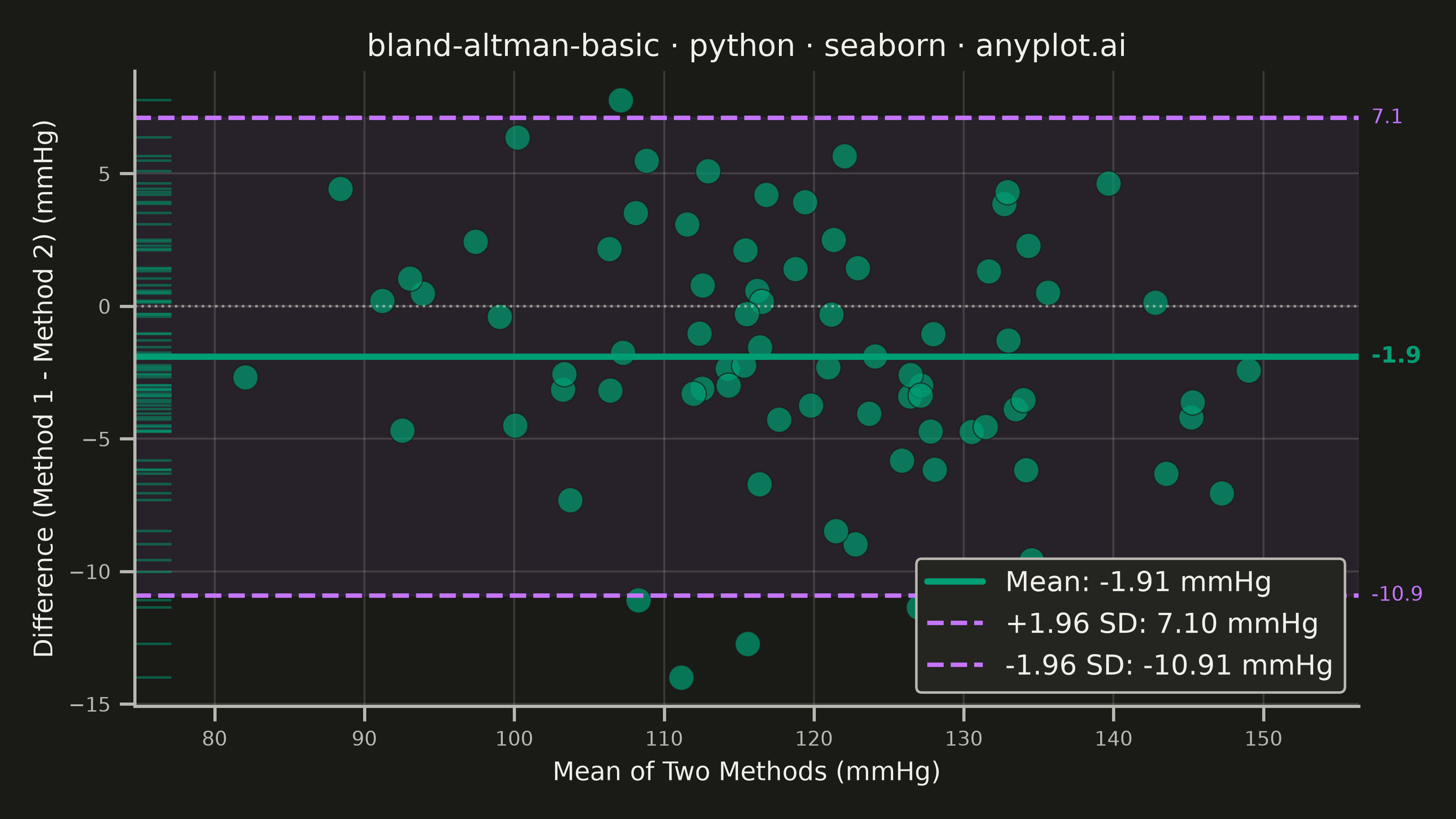
A Bland-Altman plot (also known as a difference plot or Tukey mean-difference plot) visualizes the agreement between two measurement methods by plotting the difference against the average of paired observations. It displays the mean difference (bias) as a horizontal line and limits of agreement (mean ± 1.96 SD) to assess whether the methods are interchangeable within acceptable tolerances.
""" anyplot.ai
bland-altman-basic: Bland-Altman Agreement Plot
Library: seaborn 0.13.2 | Python 3.13.14
Quality: 90/100 | Updated: 2026-08-11
"""

import os
import sys


# Remove current directory from path to avoid importing this file as 'seaborn'
sys.path = [p for p in sys.path if os.path.abspath(p) != os.getcwd()]

import matplotlib.pyplot as plt
import numpy as np
import seaborn as sns


# Theme tokens
THEME = os.getenv("ANYPLOT_THEME", "light")
PAGE_BG = "#FAF8F1" if THEME == "light" else "#1A1A17"
ELEVATED_BG = "#FFFDF6" if THEME == "light" else "#242420"
INK = "#1A1A17" if THEME == "light" else "#F0EFE8"
INK_SOFT = "#4A4A44" if THEME == "light" else "#B8B7B0"

# Imprint palette (categorical) — first series always #009E73
IMPRINT_PALETTE = sns.color_palette(["#009E73", "#C475FD"])
BRAND = IMPRINT_PALETTE[0]  # scatter + mean line
ACCENT_1 = IMPRINT_PALETTE[1]  # limits of agreement
NEUTRAL = INK  # semantic anchor: baseline / reference line, same hex as text

# Theme-adaptive chrome, seaborn-native (see prompts/library/seaborn.md)
sns.set_theme(
    style="ticks",
    rc={
        "figure.facecolor": PAGE_BG,
        "axes.facecolor": PAGE_BG,
        "axes.edgecolor": INK_SOFT,
        "axes.labelcolor": INK,
        "text.color": INK,
        "xtick.color": INK_SOFT,
        "ytick.color": INK_SOFT,
        "grid.color": INK,
        "grid.alpha": 0.15,
        "legend.facecolor": ELEVATED_BG,
        "legend.edgecolor": INK_SOFT,
    },
)

# Data - Simulated blood pressure measurements from two sphygmomanometers
np.random.seed(42)
n = 80

# Method 1: Reference standard (e.g., mercury sphygmomanometer)
method1 = np.random.normal(120, 15, n)

# Method 2: New device with slight systematic bias and proportional error
method2 = method1 + np.random.normal(2, 5, n) + 0.02 * (method1 - 120)

# Calculate Bland-Altman statistics
mean_values = (method1 + method2) / 2
differences = method1 - method2
mean_diff = np.mean(differences)
std_diff = np.std(differences, ddof=1)
upper_loa = mean_diff + 1.96 * std_diff
lower_loa = mean_diff - 1.96 * std_diff

# Create plot — canonical landscape canvas (3200x1800 @ dpi=400)
fig, ax = plt.subplots(figsize=(8, 4.5), dpi=400)

# Scatter plot of differences vs means
sns.scatterplot(x=mean_values, y=differences, s=100, alpha=0.7, color=BRAND, edgecolor=PAGE_BG, linewidth=0.5, ax=ax)

# Rug of the raw differences on the y-axis — a seaborn-native way to surface
# the shape of the difference distribution, which the ±1.96 SD limits assume
# is approximately normal.
sns.rugplot(y=differences, ax=ax, height=0.03, color=BRAND, alpha=0.5, lw=1)

# Shaded band between the limits of agreement — reinforces the ±1.96 SD
# envelope as a single focal region before the individual lines are read.
ax.axhspan(lower_loa, upper_loa, color=ACCENT_1, alpha=0.08, zorder=0)

# Mean difference line (bias)
ax.axhline(y=mean_diff, color=BRAND, linewidth=2.5, label=f"Mean: {mean_diff:.2f} mmHg")

# Limits of agreement (±1.96 SD)
ax.axhline(y=upper_loa, color=ACCENT_1, linewidth=1.75, linestyle="--", label=f"+1.96 SD: {upper_loa:.2f} mmHg")
ax.axhline(y=lower_loa, color=ACCENT_1, linewidth=1.75, linestyle="--", label=f"-1.96 SD: {lower_loa:.2f} mmHg")

# Zero reference line
ax.axhline(y=0, color=NEUTRAL, linewidth=1, linestyle=":", alpha=0.5)

# Annotate values on the right side
x_max = ax.get_xlim()[1]
ax.annotate(
    f"{mean_diff:.1f}",
    xy=(x_max, mean_diff),
    xytext=(5, 0),
    textcoords="offset points",
    fontsize=9,
    color=BRAND,
    fontweight="bold",
    va="center",
)
ax.annotate(
    f"{upper_loa:.1f}",
    xy=(x_max, upper_loa),
    xytext=(5, 0),
    textcoords="offset points",
    fontsize=8,
    color=ACCENT_1,
    va="center",
)
ax.annotate(
    f"{lower_loa:.1f}",
    xy=(x_max, lower_loa),
    xytext=(5, 0),
    textcoords="offset points",
    fontsize=8,
    color=ACCENT_1,
    va="center",
)

# Labels and styling
ax.set_xlabel("Mean of Two Methods (mmHg)", fontsize=10)
ax.set_ylabel("Difference (Method 1 - Method 2) (mmHg)", fontsize=10)
ax.set_title("bland-altman-basic · python · seaborn · anyplot.ai", fontsize=12, fontweight="medium")
ax.tick_params(axis="both", labelsize=8)

# Spines — seaborn-native despine (default: top + right removed)
sns.despine(ax=ax)

# Grid - subtle, both axes (scatter plot)
ax.grid(True, axis="both", alpha=0.15, linewidth=0.8, color=INK)

# Legend, positioned and styled via seaborn's move_legend — lower-right,
# clear of both the y-axis rug ticks and the right-edge value annotations
ax.legend(fontsize=8)
sns.move_legend(ax, "lower right", frameon=True, facecolor=ELEVATED_BG, edgecolor=INK_SOFT, framealpha=1.0)

plt.tight_layout()
plt.savefig(f"plot-{THEME}.png", dpi=400, facecolor=PAGE_BG)
Runnable source as JSON, for any HTTP client: https://api.anyplot.ai/specs/bland-altman-basic/seaborn/code. Any spec id and library id listed in llms-full.txt fit the same URL shape; every URL below is complete and callable.
{
  "spec_id": "bland-altman-basic",
  "language": "python",
  "library": "seaborn",
  "page": "https://anyplot.ai/bland-altman-basic/python/seaborn",
  "hub": "https://anyplot.ai/bland-altman-basic",
  "code_json": "https://api.anyplot.ai/specs/bland-altman-basic/seaborn/code",
  "spec_json": "https://api.anyplot.ai/specs/bland-altman-basic",
  "render_light_png": "https://storage.googleapis.com/anyplot-images/plots/bland-altman-basic/python/seaborn/plot-light.png",
  "render_dark_png": "https://storage.googleapis.com/anyplot-images/plots/bland-altman-basic/python/seaborn/plot-dark.png",
  "quality_score": 90.0,
  "license": "MIT",
  "guide": "https://anyplot.ai/llms.txt"
}
Part of Bland-Altman Agreement Plot on anyplot.ai.