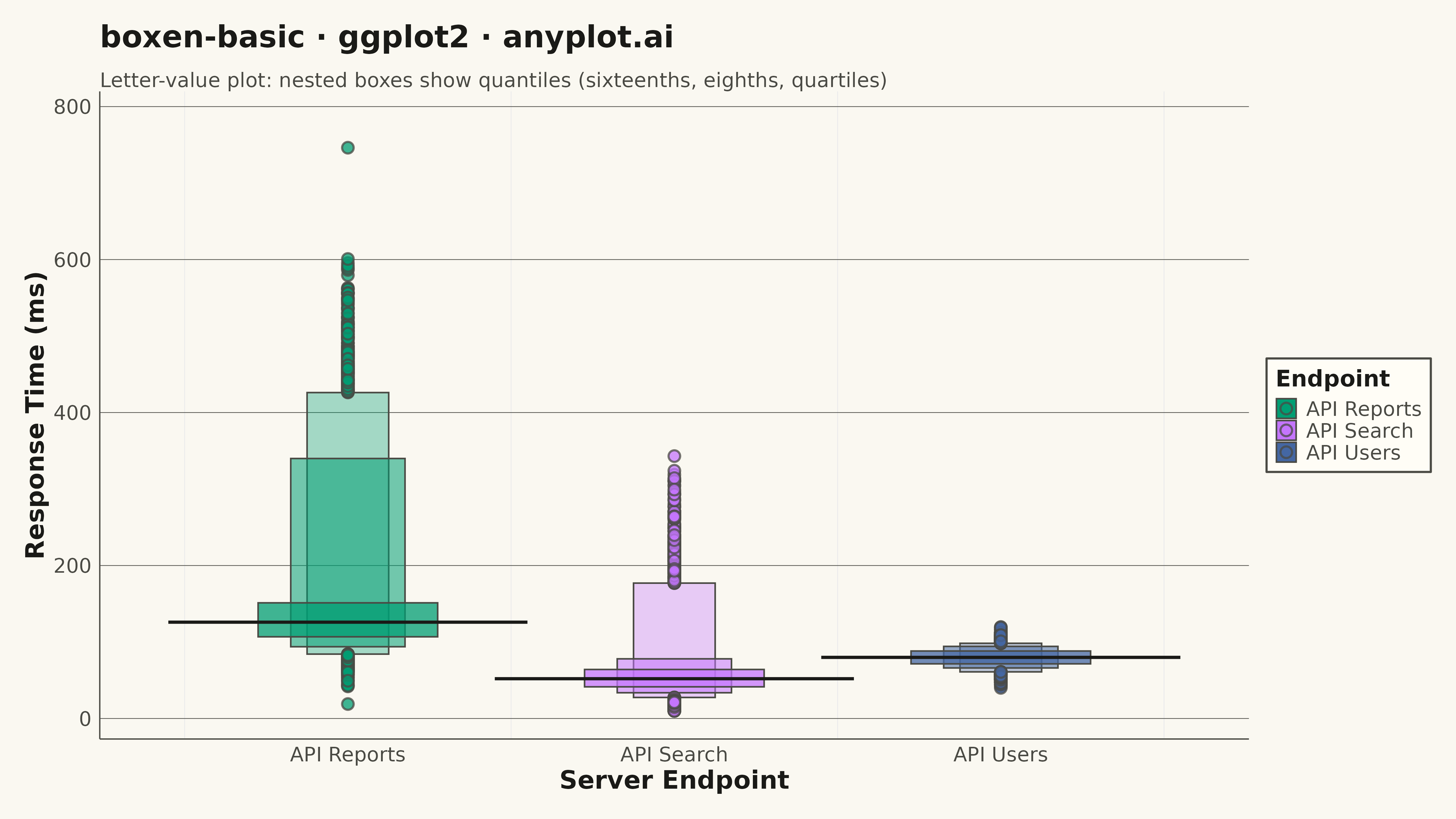
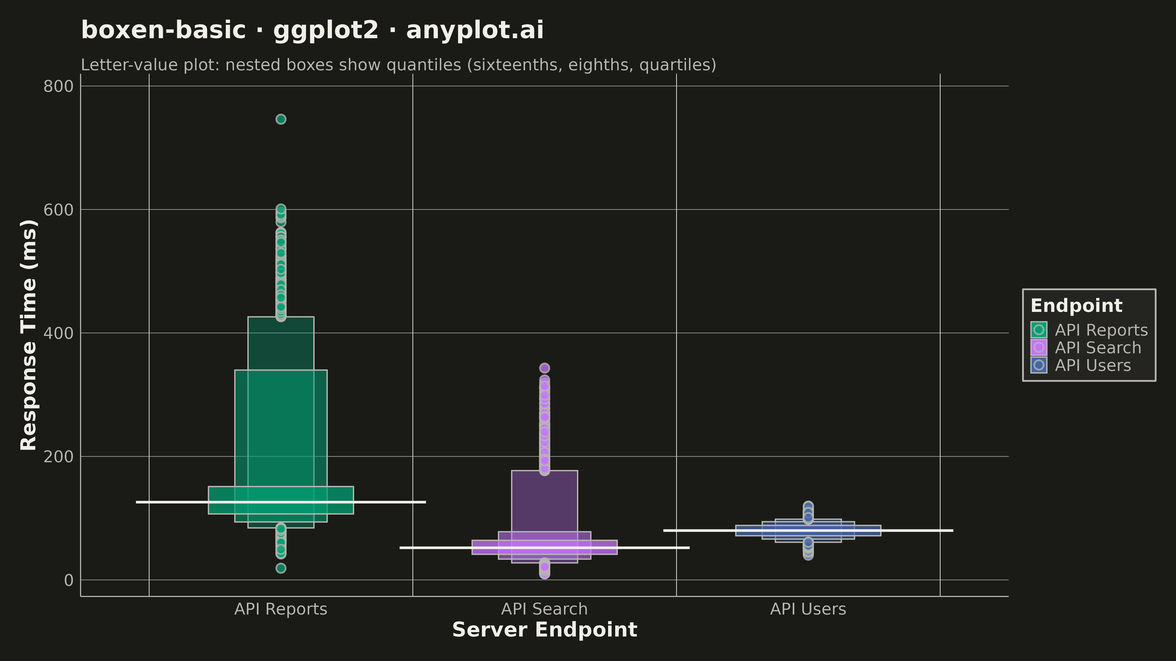
The same plot in 14 other libraries — Python: Altair, Bokeh, lets-plot, Matplotlib, Plotly, plotnine, Pygal, Seaborn; Julia: Makie.jl; JavaScript: Chart.js, D3.js, Apache ECharts, Highcharts, MUI X Charts. Compare all 15 side by side: Basic Boxen Plot (Letter-Value Plot) in Python, R, Julia and JavaScript.
A boxen plot (also known as letter-value plot) extends the traditional box plot to show more quantile information, making it ideal for large datasets with 1000+ observations. Instead of just displaying the median and quartiles, it shows additional "letter values" (eighths, sixteenths, etc.) as nested boxes, revealing the full shape of the distribution including tail behavior. This makes outlier detection more meaningful and distribution comparison more detailed.
#' anyplot.ai
#' boxen-basic: Basic Boxen Plot (Letter-Value Plot)
#' Library: ggplot2 3.5.1 | R 4.4.1
#' Quality: 91/100 | Created: 2026-05-17

library(ggplot2)
library(dplyr)
library(ragg)
library(tibble)

set.seed(42)

# --- Theme tokens -----------------------------------------------------------
THEME       <- Sys.getenv("ANYPLOT_THEME", "light")
PAGE_BG     <- if (THEME == "light") "#FAF8F1" else "#1A1A17"
ELEVATED_BG <- if (THEME == "light") "#FFFDF6" else "#242420"
INK         <- if (THEME == "light") "#1A1A17" else "#F0EFE8"
INK_SOFT    <- if (THEME == "light") "#4A4A44" else "#B8B7B0"
IMPRINT   <- c("#009E73", "#C475FD", "#4467A3", "#BD8233",
                 "#AE3030", "#2ABCCD", "#954477")

# --- Data -------------------------------------------------------------------
# Simulate response time distributions across three server endpoints
set.seed(42)

df <- tibble(
  endpoint = c(
    rep("API Search", 3000),
    rep("API Users", 3000),
    rep("API Reports", 3000)
  ),
  response_time_ms = c(
    c(rnorm(2700, mean = 50, sd = 15), rnorm(300, mean = 200, sd = 50)),
    rnorm(3000, mean = 80, sd = 12),
    c(rnorm(2500, mean = 120, sd = 25), rnorm(500, mean = 400, sd = 80))
  )
) %>%
  mutate(response_time_ms = pmax(response_time_ms, 10))

# --- Letter-Value Plot Construction -------------------------------------------
# Compute quantiles at multiple levels for nested boxes: median, quartiles, eighths, sixteenths
compute_letter_values <- function(x) {
  tibble(
    level = c(4, 3, 2, 1, 0),  # sixteenths, eighths, quartiles, median, outliers
    q_low = c(
      quantile(x, 0.0625, na.rm = TRUE),   # 1/16
      quantile(x, 0.125, na.rm = TRUE),    # 1/8
      quantile(x, 0.25, na.rm = TRUE),     # 1/4
      quantile(x, 0.5, na.rm = TRUE),      # median
      quantile(x, 0.5, na.rm = TRUE)
    ),
    q_high = c(
      quantile(x, 0.9375, na.rm = TRUE),   # 15/16
      quantile(x, 0.875, na.rm = TRUE),    # 7/8
      quantile(x, 0.75, na.rm = TRUE),     # 3/4
      quantile(x, 0.5, na.rm = TRUE),      # median
      quantile(x, 0.5, na.rm = TRUE)
    ),
    width_frac = c(0.25, 0.35, 0.55, 1.0, 0)
  )
}

# Generate letter-value data for all groups
lv_data <- df %>%
  group_by(endpoint) %>%
  reframe(compute_letter_values(response_time_ms))

# Identify outliers beyond sixteenths
outlier_data <- df %>%
  group_by(endpoint) %>%
  summarize(
    q_low_16 = quantile(response_time_ms, 0.0625, na.rm = TRUE),
    q_high_16 = quantile(response_time_ms, 0.9375, na.rm = TRUE),
    .groups = "drop"
  ) %>%
  inner_join(
    df,
    by = "endpoint"
  ) %>%
  filter(response_time_ms < q_low_16 | response_time_ms > q_high_16) %>%
  select(endpoint, response_time_ms)

# --- Plot -------------------------------------------------------------------
# Establish x-position and width mapping
endpoints <- unique(lv_data$endpoint)
x_pos <- seq_along(endpoints)
names(x_pos) <- endpoints

p <- ggplot() +
  # Layer 1: Nested boxes (sixteenths, eighths, quartiles, median)
  geom_rect(
    data = lv_data %>% filter(level > 0),
    aes(
      xmin = as.numeric(factor(endpoint, levels = endpoints)) - 0.5 * width_frac,
      xmax = as.numeric(factor(endpoint, levels = endpoints)) + 0.5 * width_frac,
      ymin = q_low,
      ymax = q_high,
      fill = endpoint,
      alpha = rev(0.15 + 0.2 * level)  # Darker/opaque for inner boxes
    ),
    color = INK_SOFT,
    linewidth = 0.6
  ) +
  # Layer 2: Median line
  geom_segment(
    data = lv_data %>% filter(level == 1),
    aes(
      x = as.numeric(factor(endpoint, levels = endpoints)) - 0.55,
      xend = as.numeric(factor(endpoint, levels = endpoints)) + 0.55,
      y = q_low,
      yend = q_low
    ),
    color = INK,
    linewidth = 1.2
  ) +
  # Layer 3: Outliers
  geom_point(
    data = outlier_data,
    aes(
      x = as.numeric(factor(endpoint, levels = endpoints)),
      y = response_time_ms,
      fill = endpoint
    ),
    size = 3.5,
    shape = 21,
    color = INK_SOFT,
    stroke = 1.2,
    alpha = 0.75
  ) +
  scale_fill_manual(
    name = "Endpoint",
    values = IMPRINT[1:3],
    breaks = endpoints
  ) +
  scale_alpha_identity() +
  scale_x_continuous(
    breaks = x_pos,
    labels = names(x_pos),
    limits = c(0.4, length(endpoints) + 0.6)
  ) +
  scale_y_continuous(expand = expansion(mult = c(0.05, 0.1))) +
  labs(
    title = "boxen-basic · ggplot2 · anyplot.ai",
    subtitle = "Letter-value plot: nested boxes show quantiles (sixteenths, eighths, quartiles)",
    x = "Server Endpoint",
    y = "Response Time (ms)"
  ) +
  theme_minimal(base_size = 14) +
  theme(
    plot.background   = element_rect(fill = PAGE_BG, color = PAGE_BG),
    panel.background  = element_rect(fill = PAGE_BG, color = NA),
    panel.grid.major.x = element_blank(),
    panel.grid.minor.y = element_blank(),
    panel.grid.major.y = element_line(color = INK_SOFT, linewidth = 0.25),
    panel.border      = element_blank(),
    axis.line.x       = element_line(color = INK_SOFT, linewidth = 0.5),
    axis.line.y       = element_line(color = INK_SOFT, linewidth = 0.5),
    axis.title        = element_text(color = INK, size = 20, face = "bold"),
    axis.text         = element_text(color = INK_SOFT, size = 16),
    plot.title        = element_text(color = INK, size = 24, face = "bold"),
    plot.subtitle     = element_text(color = INK_SOFT, size = 16, margin = margin(t = 8)),
    legend.position   = "right",
    legend.background = element_rect(fill = ELEVATED_BG, color = INK_SOFT, linewidth = 0.8),
    legend.text       = element_text(color = INK_SOFT, size = 16),
    legend.title      = element_text(color = INK, size = 18, face = "bold"),
    legend.key        = element_blank(),
    plot.margin       = margin(20, 20, 20, 20, "pt")
  )

# --- Save -------------------------------------------------------------------
ggsave(
  filename = sprintf("plot-%s.png", THEME),
  plot     = p,
  device   = ragg::agg_png,
  width    = 16,
  height   = 9,
  units    = "in",
  dpi      = 300
)
Runnable source as JSON, for any HTTP client: https://api.anyplot.ai/specs/boxen-basic/ggplot2/code. Any spec id and library id listed in llms-full.txt fit the same URL shape; every URL below is complete and callable.
{
  "spec_id": "boxen-basic",
  "language": "r",
  "library": "ggplot2",
  "page": "https://anyplot.ai/boxen-basic/r/ggplot2",
  "hub": "https://anyplot.ai/boxen-basic",
  "code_json": "https://api.anyplot.ai/specs/boxen-basic/ggplot2/code",
  "spec_json": "https://api.anyplot.ai/specs/boxen-basic",
  "render_light_png": "https://storage.googleapis.com/anyplot-images/plots/boxen-basic/r/ggplot2/plot-light.png",
  "render_dark_png": "https://storage.googleapis.com/anyplot-images/plots/boxen-basic/r/ggplot2/plot-dark.png",
  "quality_score": 91.0,
  "license": "MIT",
  "guide": "https://anyplot.ai/llms.txt"
}
Part of Basic Boxen Plot (Letter-Value Plot) on anyplot.ai.