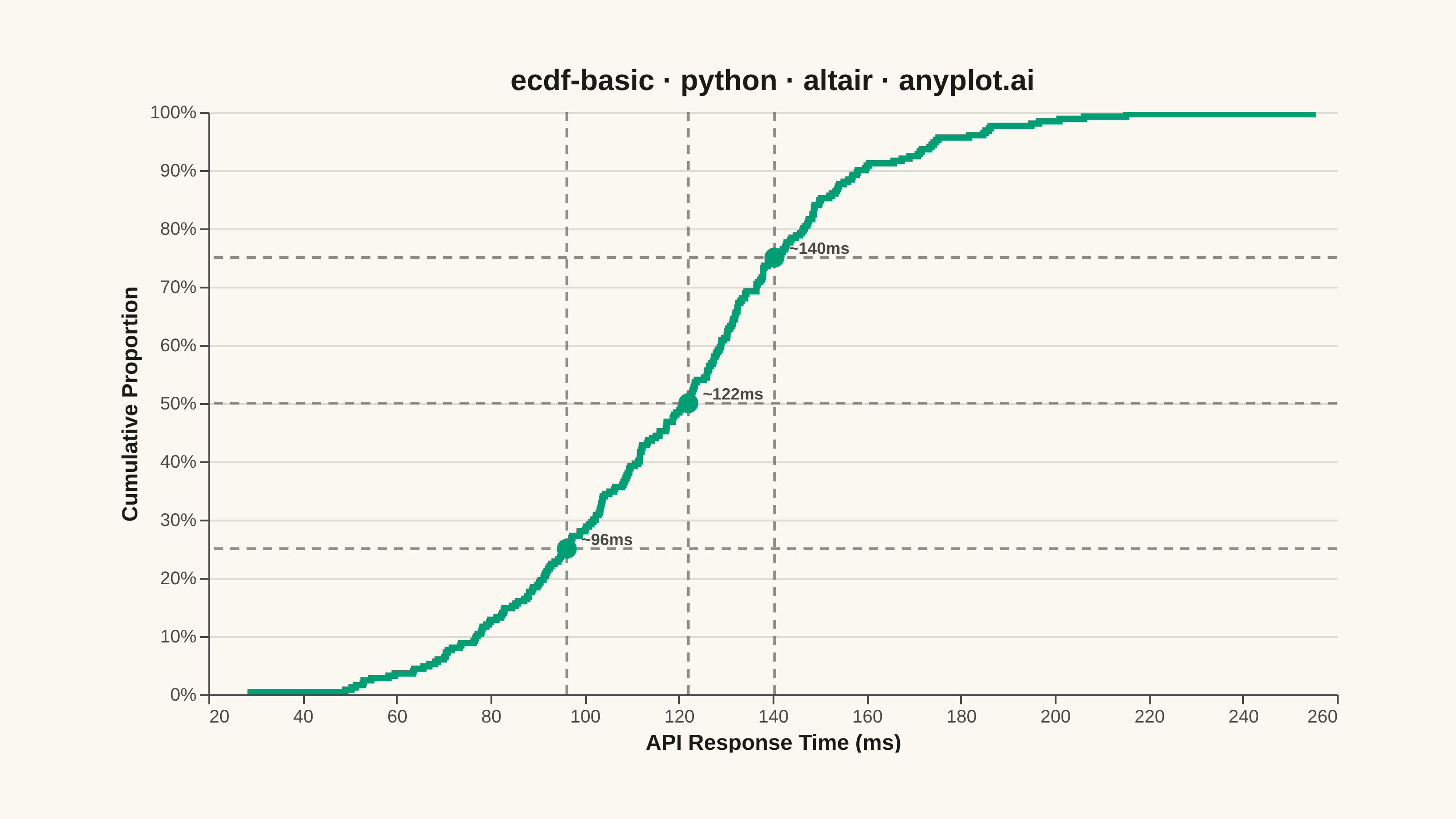
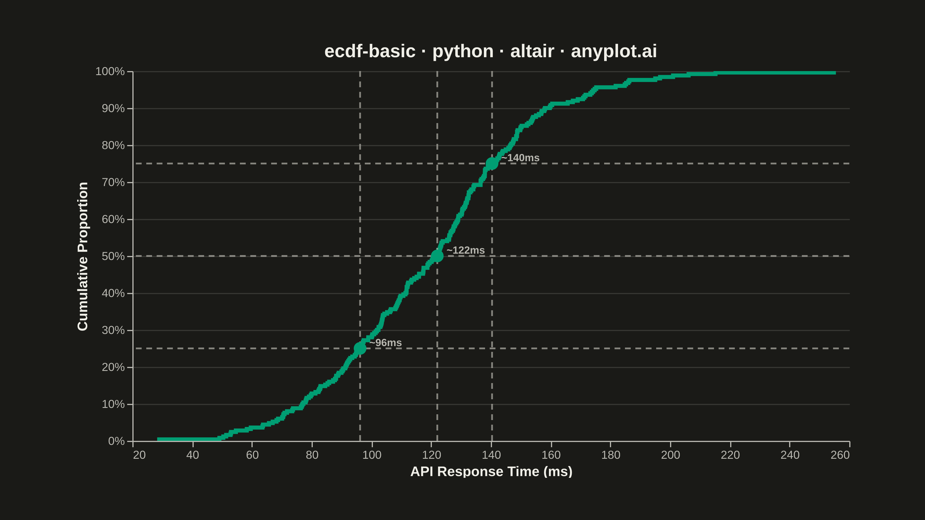
An ECDF (Empirical Cumulative Distribution Function) plot displays a step function that shows the proportion of observations less than or equal to each value. Unlike histograms, ECDF plots require no binning or smoothing, providing a non-parametric estimate of the cumulative distribution. The y-axis ranges from 0 to 1, allowing direct reading of percentiles and quantiles from the visualization.
""" anyplot.ai
ecdf-basic: Basic ECDF Plot
Library: altair 6.2.2 | Python 3.13.14
Quality: 90/100 | Updated: 2026-06-25
"""

import os
import sys


# The file is named altair.py; remove its own directory from sys.path so
# `import altair` resolves to the library, not this script.
_HERE = os.path.dirname(os.path.abspath(__file__))
sys.path = [p for p in sys.path if not p or os.path.abspath(p) != _HERE]
os.chdir(_HERE)  # saves (plot-*.png, plot-*.html) land in the implementations dir

import altair as alt
import numpy as np
import pandas as pd
from PIL import Image


# Theme tokens
THEME = os.getenv("ANYPLOT_THEME", "light")
PAGE_BG = "#FAF8F1" if THEME == "light" else "#1A1A17"
ELEVATED_BG = "#FFFDF6" if THEME == "light" else "#242420"
INK = "#1A1A17" if THEME == "light" else "#F0EFE8"
INK_SOFT = "#4A4A44" if THEME == "light" else "#B8B7B0"
INK_MUTED = "#6B6A63" if THEME == "light" else "#A8A79F"
BRAND = "#009E73"  # Imprint palette position 1 — always first series

# Data: API response latency from a production web service
np.random.seed(42)
response_times_ms = np.random.normal(loc=120, scale=35, size=250)
response_times_ms = np.clip(response_times_ms, 20, None)

# Raw data frame — ECDF computed declaratively via Vega-Lite window transform
df = pd.DataFrame({"latency_ms": response_times_ms})

# Reference values at quartiles for focal emphasis and text annotations
p25_ms = float(np.percentile(response_times_ms, 25))
p50_ms = float(np.median(response_times_ms))
p75_ms = float(np.percentile(response_times_ms, 75))
ref_df = pd.DataFrame(
    {
        "latency_ms": [p25_ms, p50_ms, p75_ms],
        "cumulative": [0.25, 0.50, 0.75],
        "label": [f"~{p25_ms:.0f}ms", f"~{p50_ms:.0f}ms", f"~{p75_ms:.0f}ms"],
    }
)

# Title
title_str = "ecdf-basic · python · altair · anyplot.ai"

# ECDF step function — cume_dist() window transform computes the ECDF declaratively
# in Vega-Lite without numpy preprocessing; step-after gives the correct step shape
ecdf_line = (
    alt.Chart(df)
    .transform_window(ecdf="cume_dist()", sort=[alt.SortField("latency_ms")])
    .mark_line(interpolate="step-after", strokeWidth=3.5, color=BRAND)
    .encode(
        x=alt.X("latency_ms:Q", title="API Response Time (ms)", scale=alt.Scale(nice=True)),
        y=alt.Y(
            "ecdf:Q",
            title="Cumulative Proportion",
            scale=alt.Scale(domain=[0, 1]),
            axis=alt.Axis(format=".0%", tickCount=11),
        ),
        tooltip=[
            alt.Tooltip("latency_ms:Q", title="Latency (ms)", format=".1f"),
            alt.Tooltip("ecdf:Q", title="Proportion", format=".3f"),
        ],
    )
)

# Dashed reference lines spanning the full axes at Q1, median, Q3
h_rules = (
    alt.Chart(ref_df)
    .mark_rule(strokeDash=[5, 4], strokeWidth=1.5, color=INK_MUTED, opacity=0.75)
    .encode(y="cumulative:Q")
)

v_rules = (
    alt.Chart(ref_df)
    .mark_rule(strokeDash=[5, 4], strokeWidth=1.5, color=INK_MUTED, opacity=0.75)
    .encode(x="latency_ms:Q")
)

# Focal markers at quartile intersections on the ECDF
focal_pts = (
    alt.Chart(ref_df)
    .mark_point(size=120, filled=True, color=BRAND, opacity=1.0)
    .encode(
        x="latency_ms:Q",
        y="cumulative:Q",
        tooltip=[
            alt.Tooltip("latency_ms:Q", title="Latency (ms)", format=".1f"),
            alt.Tooltip("cumulative:Q", title="Quartile", format=".0%"),
        ],
    )
)

# Text annotations at focal points for at-a-glance percentile reading without hover
focal_labels = (
    alt.Chart(ref_df)
    .mark_text(align="left", dx=8, dy=-5, fontSize=9, color=INK_SOFT, fontWeight="bold")
    .encode(x="latency_ms:Q", y="cumulative:Q", text="label:N")
)

# Compose layers and configure theme-adaptive chrome
chart = (
    alt.layer(ecdf_line, h_rules, v_rules, focal_pts, focal_labels)
    .interactive()
    .properties(
        width=620,
        height=320,
        background=PAGE_BG,
        padding={"left": 0, "right": 0, "top": 0, "bottom": 0},
        title=alt.Title(title_str, fontSize=16, color=INK),
    )
    .configure_view(fill=PAGE_BG, stroke=INK_SOFT, strokeWidth=0, continuousWidth=620, continuousHeight=320)
    .configure_axis(
        domainColor=INK_SOFT,
        tickColor=INK_SOFT,
        labelColor=INK_SOFT,
        titleColor=INK,
        labelFontSize=10,
        titleFontSize=12,
    )
    .configure_axisX(grid=False)
    .configure_axisY(gridColor=INK, gridOpacity=0.13)
    .configure_title(color=INK)
)

# Save
chart.save(f"plot-{THEME}.png", scale_factor=4.0)
chart.save(f"plot-{THEME}.html")

# Canvas: pad to exactly 3200×1800 with PAGE_BG (vl-convert inner-view padding lands short)
TW, TH = 3200, 1800
_img = Image.open(f"plot-{THEME}.png").convert("RGB")
_w, _h = _img.size
if _w > TW or _h > TH:
    raise SystemExit(
        f"altair vl-convert produced {_w}×{_h}, exceeds target {TW}×{TH}. "
        f"Shrink chart .properties(width=, height=) values and re-render."
    )
if _w < TW or _h < TH:
    _canvas = Image.new("RGB", (TW, TH), PAGE_BG)
    _canvas.paste(_img, ((TW - _w) // 2, (TH - _h) // 2))
    _canvas.save(f"plot-{THEME}.png")
Runnable source as JSON, for any HTTP client: https://api.anyplot.ai/specs/ecdf-basic/altair/code. Any spec id and library id listed in llms-full.txt fit the same URL shape; every URL below is complete and callable.
{
  "spec_id": "ecdf-basic",
  "language": "python",
  "library": "altair",
  "page": "https://anyplot.ai/ecdf-basic/python/altair",
  "hub": "https://anyplot.ai/ecdf-basic",
  "code_json": "https://api.anyplot.ai/specs/ecdf-basic/altair/code",
  "spec_json": "https://api.anyplot.ai/specs/ecdf-basic",
  "render_light_png": "https://storage.googleapis.com/anyplot-images/plots/ecdf-basic/python/altair/plot-light.png",
  "render_dark_png": "https://storage.googleapis.com/anyplot-images/plots/ecdf-basic/python/altair/plot-dark.png",
  "interactive_light_html": "https://storage.googleapis.com/anyplot-images/plots/ecdf-basic/python/altair/plot-light.html",
  "interactive_dark_html": "https://storage.googleapis.com/anyplot-images/plots/ecdf-basic/python/altair/plot-dark.html",
  "quality_score": 90.0,
  "license": "MIT",
  "guide": "https://anyplot.ai/llms.txt"
}
Part of Basic ECDF Plot on anyplot.ai.