The same plot in 14 other libraries — Python: Altair, Bokeh, lets-plot, Matplotlib, Plotly, plotnine, Pygal, Seaborn; Julia: Makie.jl; JavaScript: Chart.js, D3.js, Apache ECharts, Highcharts, MUI X Charts. Compare all 15 side by side: Basic ECDF Plot in Python, R, Julia and JavaScript.
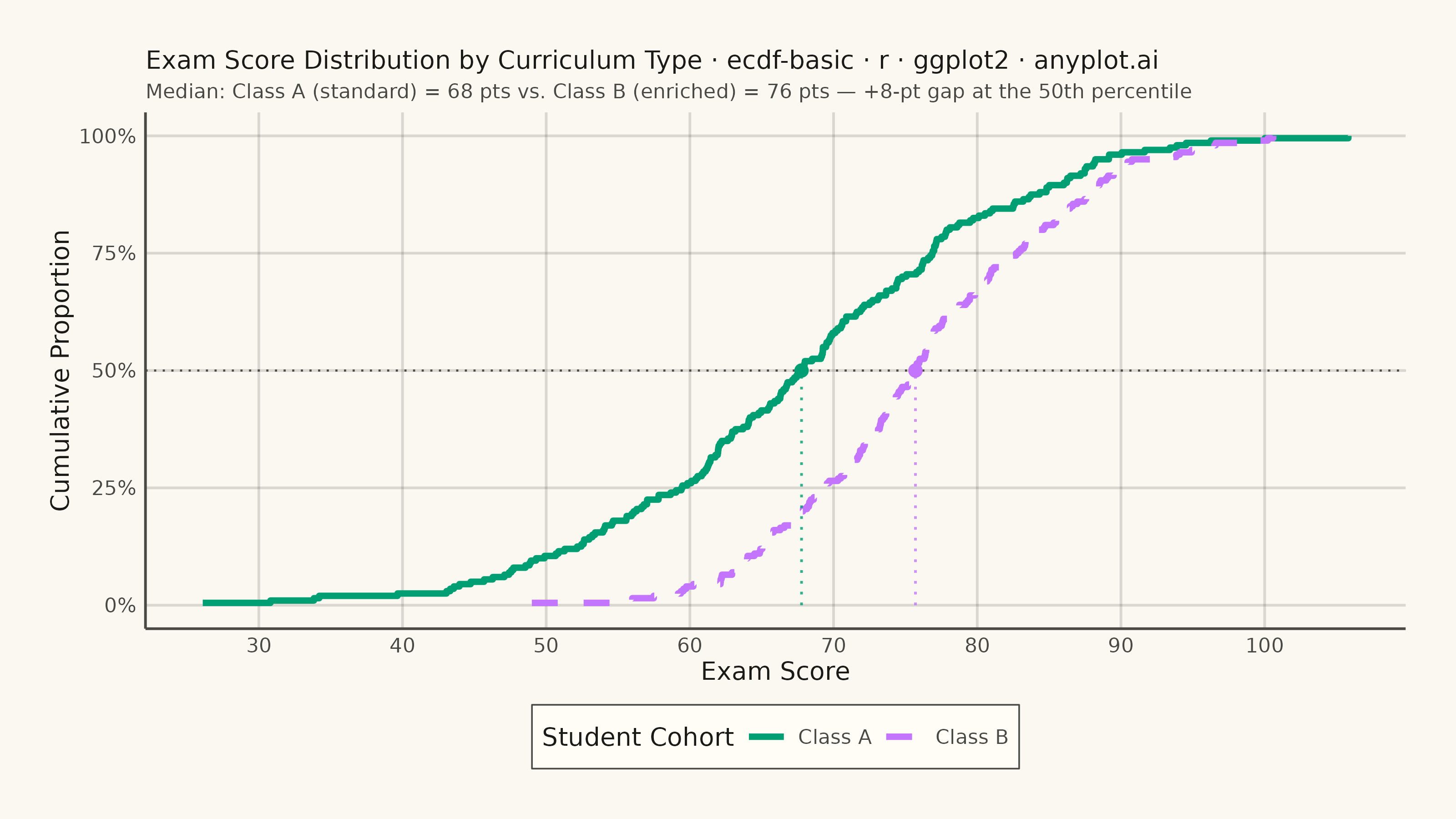
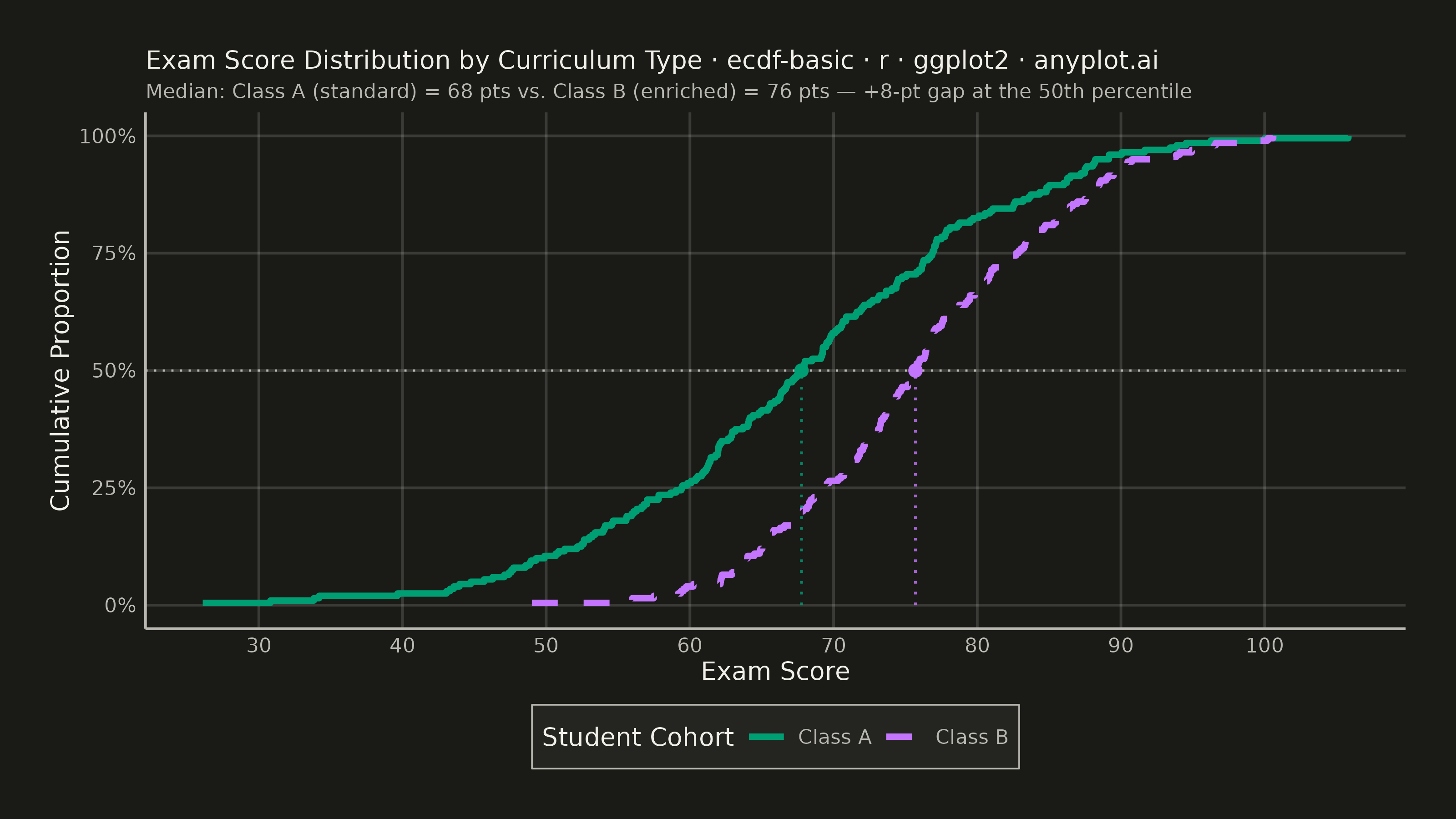
An ECDF (Empirical Cumulative Distribution Function) plot displays a step function that shows the proportion of observations less than or equal to each value. Unlike histograms, ECDF plots require no binning or smoothing, providing a non-parametric estimate of the cumulative distribution. The y-axis ranges from 0 to 1, allowing direct reading of percentiles and quantiles from the visualization.
#' anyplot.ai
#' ecdf-basic: Basic ECDF Plot
#' Library: ggplot2 3.5.1 | R 4.4.1
#' Quality: 89/100 | Created: 2026-06-25

library(ggplot2)
library(scales)
library(ragg)

set.seed(42)

# Theme tokens — Imprint palette, theme-adaptive chrome
THEME       <- Sys.getenv("ANYPLOT_THEME", "light")
PAGE_BG     <- if (THEME == "light") "#FAF8F1" else "#1A1A17"
ELEVATED_BG <- if (THEME == "light") "#FFFDF6" else "#242420"
INK         <- if (THEME == "light") "#1A1A17" else "#F0EFE8"
INK_SOFT    <- if (THEME == "light") "#4A4A44" else "#B8B7B0"
GRID_COLOR  <- if (THEME == "light") "#1A1A1726" else "#F0EFE826"

IMPRINT_PALETTE <- c(
  "#009E73",  # 1 — brand green (first categorical series)
  "#C475FD",  # 2 — lavender
  "#4467A3",  # 3 — blue
  "#BD8233",  # 4 — ochre
  "#AE3030",  # 5 — matte red
  "#2ABCCD",  # 6 — cyan
  "#954477",  # 7 — rose
  "#99B314"   # 8 — lime
)

# Data: exam scores comparing two student cohorts
n <- 200
scores_a <- rnorm(n, mean = 68, sd = 14)  # standard curriculum
scores_b <- rnorm(n, mean = 76, sd = 10)  # enriched curriculum

df <- data.frame(
  score  = c(scores_a, scores_b),
  cohort = rep(c("Class A", "Class B"), each = n)
)

# Medians for reference annotations
median_a <- median(scores_a)
median_b <- median(scores_b)
gap <- round(median_b - median_a)

# Plot
p <- ggplot(df, aes(x = score, color = cohort, linetype = cohort)) +
  # Horizontal dotted reference at 50th percentile for reading medians
  geom_hline(
    yintercept = 0.5,
    color      = INK_SOFT,
    linewidth  = 0.4,
    linetype   = "dotted"
  ) +
  # ECDF step lines
  stat_ecdf(linewidth = 1.2, pad = FALSE) +
  # Vertical droplines from x-axis to 50th percentile for each cohort
  annotate("segment",
    x = median_a, xend = median_a, y = 0, yend = 0.5,
    color = IMPRINT_PALETTE[1], linewidth = 0.5, linetype = "dotted", alpha = 0.8
  ) +
  annotate("segment",
    x = median_b, xend = median_b, y = 0, yend = 0.5,
    color = IMPRINT_PALETTE[2], linewidth = 0.5, linetype = "dotted", alpha = 0.8
  ) +
  # Markers at median intersections on each ECDF curve
  annotate("point",
    x = median_a, y = 0.5,
    color = IMPRINT_PALETTE[1], size = 2.0
  ) +
  annotate("point",
    x = median_b, y = 0.5,
    color = IMPRINT_PALETTE[2], size = 2.0
  ) +
  scale_color_manual(
    name   = "Student Cohort",
    values = c("Class A" = IMPRINT_PALETTE[1], "Class B" = IMPRINT_PALETTE[2])
  ) +
  scale_linetype_manual(
    name   = "Student Cohort",
    values = c("Class A" = "solid", "Class B" = "dashed")
  ) +
  scale_x_continuous(breaks = seq(20, 120, by = 10)) +
  scale_y_continuous(
    labels = percent_format(accuracy = 1),
    breaks = seq(0, 1, by = 0.25)
  ) +
  labs(
    title    = "Exam Score Distribution by Curriculum Type · ecdf-basic · r · ggplot2 · anyplot.ai",
    subtitle = sprintf(
      "Median: Class A (standard) = %.0f pts vs. Class B (enriched) = %.0f pts — %+.0f-pt gap at the 50th percentile",
      median_a, median_b, gap
    ),
    x = "Exam Score",
    y = "Cumulative Proportion"
  ) +
  theme_minimal(base_size = 8) +
  theme(
    plot.background   = element_rect(fill = PAGE_BG, color = PAGE_BG),
    panel.background  = element_rect(fill = PAGE_BG, color = NA),
    panel.grid.major  = element_line(color = GRID_COLOR, linewidth = 0.5),
    panel.grid.minor  = element_blank(),
    panel.border      = element_blank(),
    axis.title        = element_text(color = INK, size = 10),
    axis.text         = element_text(color = INK_SOFT, size = 8),
    axis.line         = element_line(color = INK_SOFT, linewidth = 0.5),
    plot.title        = element_text(color = INK, size = 10),
    plot.subtitle     = element_text(color = INK_SOFT, size = 8),
    legend.background = element_rect(fill = ELEVATED_BG, color = INK_SOFT, linewidth = 0.3),
    legend.text       = element_text(color = INK_SOFT, size = 8),
    legend.title      = element_text(color = INK, size = 10),
    legend.position   = "bottom",
    plot.margin       = margin(20, 20, 20, 20)
  )

# Save
ggsave(
  filename = sprintf("plot-%s.png", THEME),
  plot     = p,
  device   = ragg::agg_png,
  width    = 8,
  height   = 4.5,
  units    = "in",
  dpi      = 400
)
Runnable source as JSON, for any HTTP client: https://api.anyplot.ai/specs/ecdf-basic/ggplot2/code. Any spec id and library id listed in llms-full.txt fit the same URL shape; every URL below is complete and callable.
{
  "spec_id": "ecdf-basic",
  "language": "r",
  "library": "ggplot2",
  "page": "https://anyplot.ai/ecdf-basic/r/ggplot2",
  "hub": "https://anyplot.ai/ecdf-basic",
  "code_json": "https://api.anyplot.ai/specs/ecdf-basic/ggplot2/code",
  "spec_json": "https://api.anyplot.ai/specs/ecdf-basic",
  "render_light_png": "https://storage.googleapis.com/anyplot-images/plots/ecdf-basic/r/ggplot2/plot-light.png",
  "render_dark_png": "https://storage.googleapis.com/anyplot-images/plots/ecdf-basic/r/ggplot2/plot-dark.png",
  "quality_score": 89.0,
  "license": "MIT",
  "guide": "https://anyplot.ai/llms.txt"
}
Part of Basic ECDF Plot on anyplot.ai.