The same plot in 14 other libraries — Python: Altair, Bokeh, lets-plot, Matplotlib, Plotly, plotnine, Pygal, Seaborn; Julia: Makie.jl; JavaScript: Chart.js, D3.js, Apache ECharts, Highcharts, MUI X Charts. Compare all 15 side by side: Circular Maze Puzzle in Python, R, Julia and JavaScript.
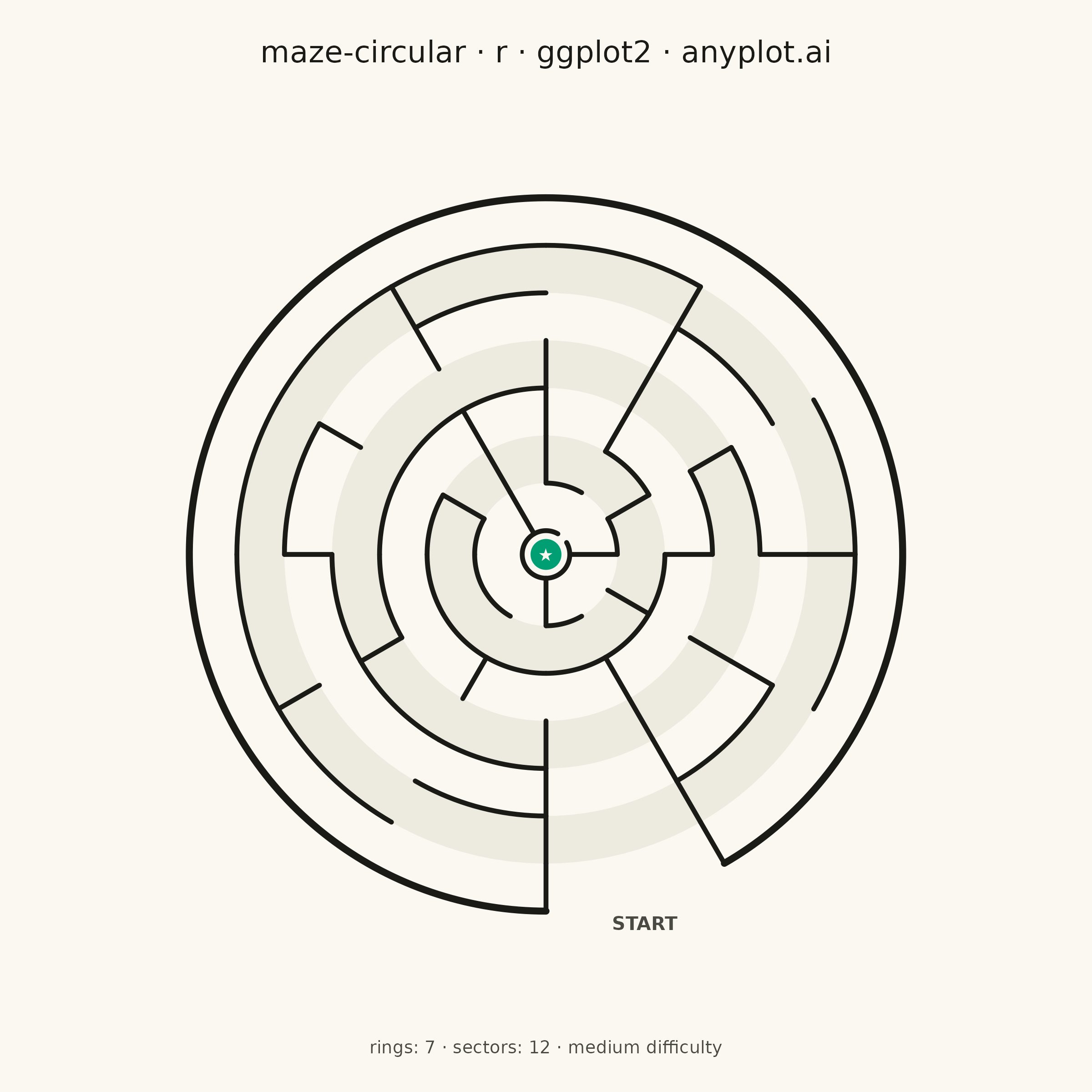
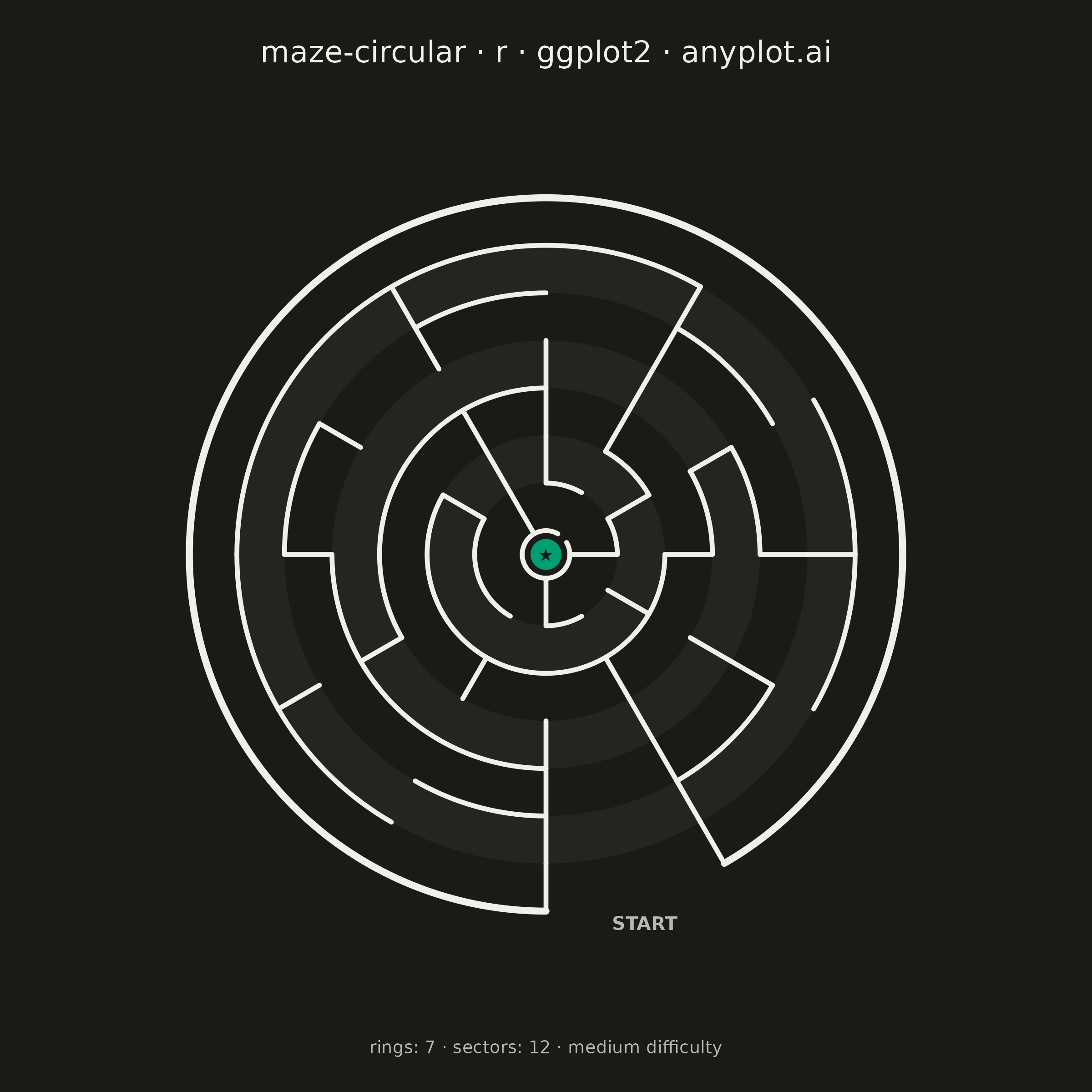
A circular maze puzzle visualization featuring concentric rings connected by radial passages. Unlike rectangular mazes, this design creates a unique solving experience where the player navigates inward through ring-shaped corridors. The maze has an entry point on the outer edge and a goal at the center, with algorithmically generated walls ensuring exactly one solvable path.
#' anyplot.ai
#' maze-circular: Circular Maze Puzzle
#' Library: ggplot2 3.5.1 | R 4.4.1
#' Quality: 90/100 | Created: 2026-05-20

library(ggplot2)
library(ragg)

set.seed(42)

# --- Theme tokens
THEME    <- Sys.getenv("ANYPLOT_THEME", "light")
PAGE_BG  <- if (THEME == "light") "#FAF8F1" else "#1A1A17"
INK      <- if (THEME == "light") "#1A1A17" else "#F0EFE8"
INK_SOFT <- if (THEME == "light") "#4A4A44" else "#B8B7B0"
BAND_ALT <- if (THEME == "light") "#EDEAE0" else "#242420"

# --- Maze parameters
RINGS        <- 7
SECTORS      <- 12
ANGLE_STEP   <- 2 * pi / SECTORS
CENTER_R     <- 0.5
ENTRY_SECTOR <- 1

ring_in  <- function(r) CENTER_R + (r - 1)
ring_out <- function(r) CENTER_R + r
OUTER_R  <- ring_out(RINGS)

sec_angle <- function(s, frac = 0) (s - 1 + frac) * ANGLE_STEP - pi / 2

# --- Iterative DFS maze generation
arc_open    <- matrix(FALSE, nrow = RINGS - 1, ncol = SECTORS)
radial_open <- matrix(FALSE, nrow = RINGS,     ncol = SECTORS)
visited     <- matrix(FALSE, nrow = RINGS,     ncol = SECTORS)

visited[RINGS, ENTRY_SECTOR] <- TRUE
dfs_stack <- list(list(r = RINGS, s = ENTRY_SECTOR))

while (length(dfs_stack) > 0) {
    top <- dfs_stack[[length(dfs_stack)]]
    r   <- top$r
    s   <- top$s
    sl  <- if (s == 1) SECTORS else s - 1
    sr  <- if (s == SECTORS) 1 else s + 1

    cands <- character(0)
    if (r > 1     && !visited[r - 1, s]) cands <- c(cands, "in")
    if (r < RINGS && !visited[r + 1, s]) cands <- c(cands, "out")
    if (!visited[r, sl])                  cands <- c(cands, "left")
    if (!visited[r, sr])                  cands <- c(cands, "right")

    if (length(cands) == 0) {
        dfs_stack <- dfs_stack[-length(dfs_stack)]
        next
    }

    dir <- sample(cands, 1)

    if (dir == "in") {
        arc_open[r - 1, s] <- TRUE
        visited[r - 1, s]  <- TRUE
        dfs_stack <- c(dfs_stack, list(list(r = r - 1, s = s)))
    } else if (dir == "out") {
        arc_open[r, s]     <- TRUE
        visited[r + 1, s]  <- TRUE
        dfs_stack <- c(dfs_stack, list(list(r = r + 1, s = s)))
    } else if (dir == "left") {
        radial_open[r, sl] <- TRUE
        visited[r, sl]     <- TRUE
        dfs_stack <- c(dfs_stack, list(list(r = r, s = sl)))
    } else {
        radial_open[r, s]  <- TRUE
        visited[r, sr]     <- TRUE
        dfs_stack <- c(dfs_stack, list(list(r = r, s = sr)))
    }
}

center_sector <- sample(seq_len(SECTORS), 1)

# --- Alternating ring band shading (visual depth: even rings tinted)
band_data <- NULL
for (r in seq_len(RINGS)) {
    if (r %% 2 == 0) {
        angs <- seq(0, 2 * pi, length.out = 120)
        ri   <- ring_in(r)
        ro   <- ring_out(r)
        df   <- data.frame(
            x    = c(ro * cos(angs), ri * cos(rev(angs))),
            y    = c(ro * sin(angs), ri * sin(rev(angs))),
            ring = r
        )
        band_data <- rbind(band_data, df)
    }
}

# --- Outer boundary (heavier stroke — visual frame, drawn separately)
outer_a0   <- sec_angle(ENTRY_SECTOR, 0)
outer_a1   <- sec_angle(ENTRY_SECTOR, 1)
outer_angs <- seq(outer_a1, outer_a0 + 2 * pi, length.out = 300)
outer_wall  <- data.frame(x = OUTER_R * cos(outer_angs), y = OUTER_R * sin(outer_angs))

# --- Accumulate inner wall geometry (center boundary + internal arcs + radial walls)
walls <- NULL
seg   <- 0L

append_seg <- function(x, y) {
    seg   <<- seg + 1L
    walls <<- rbind(walls, data.frame(x = x, y = y, seg = seg))
}

# Center boundary with goal gap
{
    a0   <- sec_angle(center_sector, 0)
    a1   <- sec_angle(center_sector, 1)
    angs <- seq(a1, a0 + 2 * pi, length.out = 180)
    append_seg(CENTER_R * cos(angs), CENTER_R * sin(angs))
}

# Internal ring boundary arcs (where wall is closed)
for (r in seq_len(RINGS - 1)) {
    wr <- ring_out(r)
    for (s in seq_len(SECTORS)) {
        if (!arc_open[r, s]) {
            angs <- seq(sec_angle(s, 0), sec_angle(s, 1), length.out = 20)
            append_seg(wr * cos(angs), wr * sin(angs))
        }
    }
}

# Radial walls (where wall is closed)
for (r in seq_len(RINGS)) {
    ri <- ring_in(r)
    ro <- ring_out(r)
    for (s in seq_len(SECTORS)) {
        if (!radial_open[r, s]) {
            angle <- sec_angle(s, 1)
            append_seg(c(ri, ro) * cos(angle), c(ri, ro) * sin(angle))
        }
    }
}

# --- Goal disc and entry label
goal_r    <- CENTER_R * 0.65
goal_angs <- seq(0, 2 * pi, length.out = 80)
goal_pts  <- data.frame(
    x = goal_r * cos(goal_angs),
    y = goal_r * sin(goal_angs)
)

entry_mid <- sec_angle(ENTRY_SECTOR, 0.5)
label_r   <- OUTER_R * 1.07
entry_lx  <- label_r * cos(entry_mid)
entry_ly  <- label_r * sin(entry_mid)

extent <- OUTER_R * 1.20

# --- Plot
p <- ggplot() +
    # Alternating ring bands for visual depth
    geom_polygon(
        data = band_data,
        aes(x = x, y = y, group = ring),
        fill = BAND_ALT, color = NA
    ) +
    # Inner walls and center boundary
    geom_path(
        data = walls,
        aes(x = x, y = y, group = factor(seg)),
        color = INK, linewidth = 0.9, lineend = "round"
    ) +
    # Outer boundary with heavier stroke for visual frame
    geom_path(
        data = outer_wall,
        aes(x = x, y = y),
        color = INK, linewidth = 1.3, lineend = "round"
    ) +
    # Goal disc
    geom_polygon(
        data = goal_pts, aes(x = x, y = y),
        fill = "#009E73", color = NA
    ) +
    annotate("text", x = 0, y = 0,
             label = "★", color = PAGE_BG, size = 2.5) +
    annotate("text", x = entry_lx, y = entry_ly,
             label = "START", color = INK_SOFT, size = 2.6,
             fontface = "bold", hjust = 0.5, vjust = 0.5) +
    coord_equal(
        xlim = c(-extent, extent),
        ylim = c(-extent, extent)
    ) +
    labs(
        title   = "maze-circular · r · ggplot2 · anyplot.ai",
        caption = "rings: 7 · sectors: 12 · medium difficulty"
    ) +
    theme_void(base_size = 8) +
    theme(
        plot.background = element_rect(fill = PAGE_BG, color = NA),
        plot.title = element_text(
            color = INK, size = 12, hjust = 0.5,
            margin = ggplot2::margin(t = 8, b = 6)
        ),
        plot.caption = element_text(
            color = INK_SOFT, size = 7, hjust = 0.5,
            margin = ggplot2::margin(t = 6, b = 6)
        ),
        plot.margin = ggplot2::margin(8, 8, 8, 8)
    )

# --- Save
ggsave(
    filename = sprintf("plot-%s.png", THEME),
    plot     = p,
    device   = ragg::agg_png,
    width    = 6,
    height   = 6,
    units    = "in",
    dpi      = 400
)
Runnable source as JSON, for any HTTP client: https://api.anyplot.ai/specs/maze-circular/ggplot2/code. Any spec id and library id listed in llms-full.txt fit the same URL shape; every URL below is complete and callable.
{
  "spec_id": "maze-circular",
  "language": "r",
  "library": "ggplot2",
  "page": "https://anyplot.ai/maze-circular/r/ggplot2",
  "hub": "https://anyplot.ai/maze-circular",
  "code_json": "https://api.anyplot.ai/specs/maze-circular/ggplot2/code",
  "spec_json": "https://api.anyplot.ai/specs/maze-circular",
  "render_light_png": "https://storage.googleapis.com/anyplot-images/plots/maze-circular/r/ggplot2/plot-light.png",
  "render_dark_png": "https://storage.googleapis.com/anyplot-images/plots/maze-circular/r/ggplot2/plot-dark.png",
  "quality_score": 90.0,
  "license": "MIT",
  "guide": "https://anyplot.ai/llms.txt"
}
Part of Circular Maze Puzzle on anyplot.ai.