The same plot in 14 other libraries — Python: Altair, Bokeh, lets-plot, Matplotlib, Plotly, plotnine, Pygal, Seaborn; Julia: Makie.jl; JavaScript: Chart.js, D3.js, Apache ECharts, Highcharts, MUI X Charts. Compare all 15 side by side: Contour Lines on Geographic Map in Python, R, Julia and JavaScript.
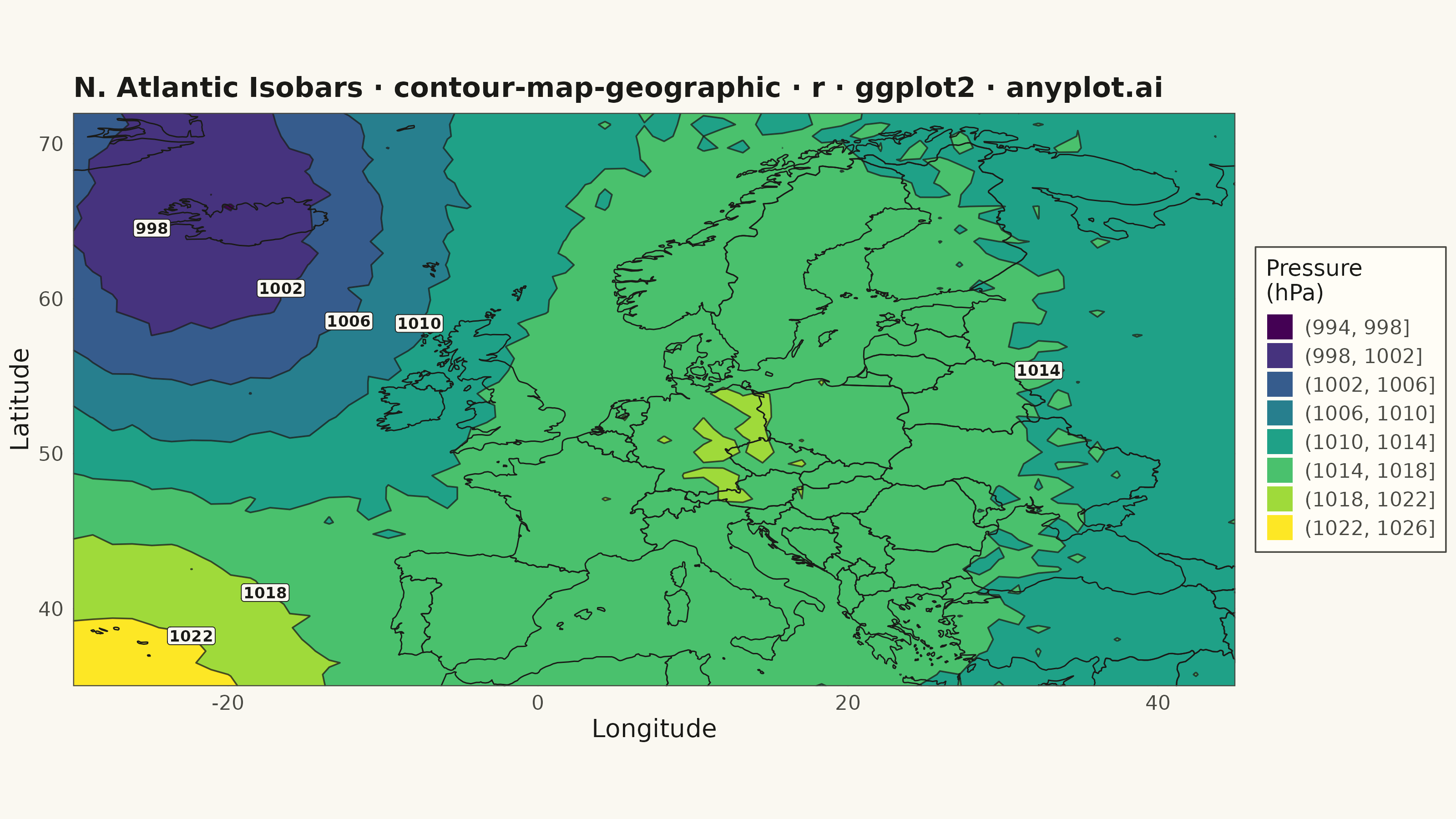
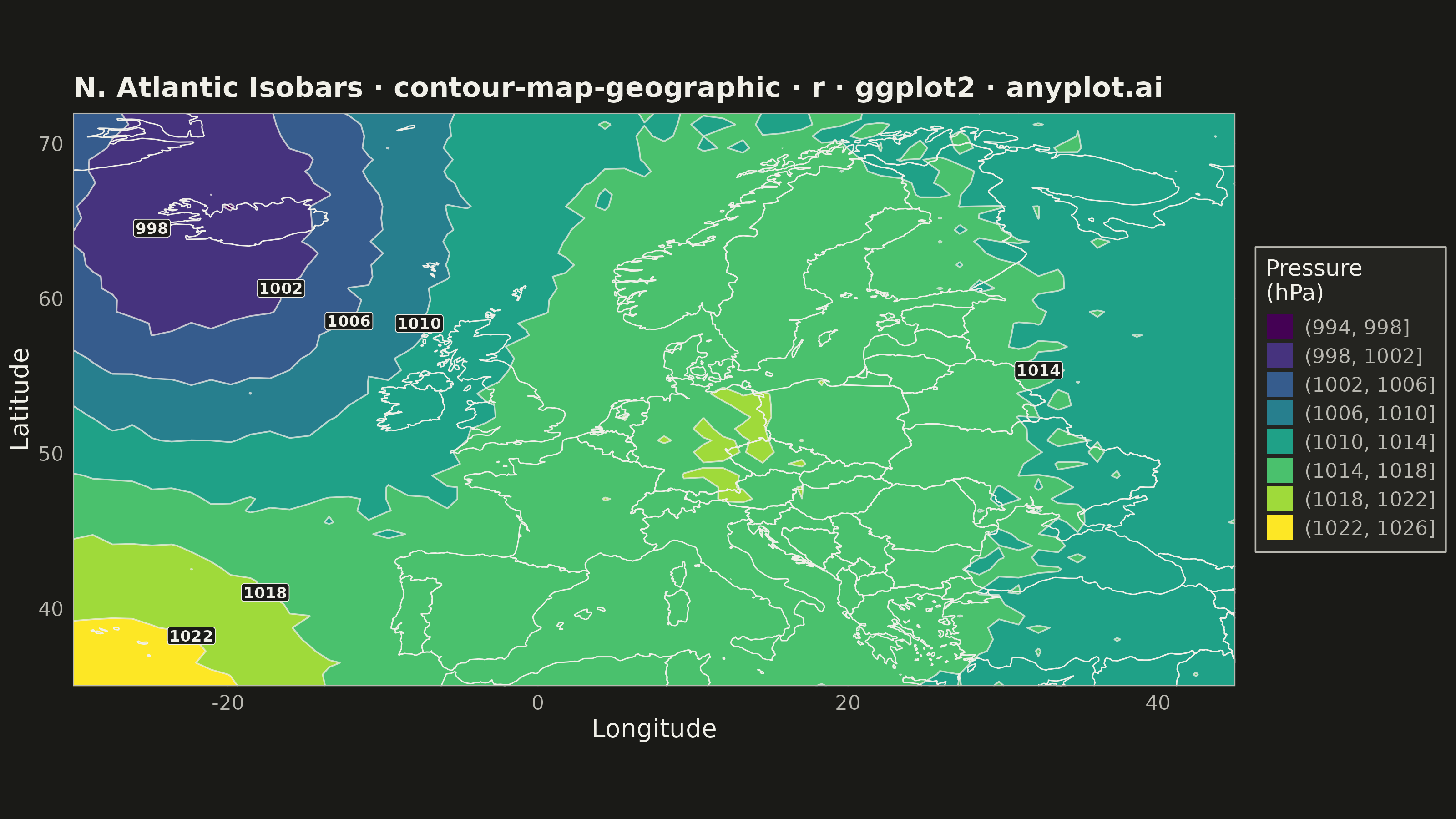
A contour map overlays isolines (lines of equal value) onto a geographic basemap, visualizing continuous spatial data such as elevation, temperature, or atmospheric pressure across real-world coordinates. Unlike basic contour plots that use abstract x/y coordinates, this plot anchors contours to latitude/longitude positions with geographic context like coastlines, borders, or terrain. It combines the precision of isoline visualization with spatial awareness, making it ideal for meteorological, topographic, and environmental applications.
#' anyplot.ai
#' contour-map-geographic: Contour Lines on Geographic Map
#' Library: ggplot2 3.5.1 | R 4.4.1
#' Quality: 92/100 | Created: 2026-05-20

library(ggplot2)
library(ragg)

set.seed(42)

# Theme tokens
THEME       <- Sys.getenv("ANYPLOT_THEME", "light")
PAGE_BG     <- if (THEME == "light") "#FAF8F1" else "#1A1A17"
ELEVATED_BG <- if (THEME == "light") "#FFFDF6" else "#242420"
INK         <- if (THEME == "light") "#1A1A17" else "#F0EFE8"
INK_SOFT    <- if (THEME == "light") "#4A4A44" else "#B8B7B0"
OCEAN_COL   <- if (THEME == "light") "#C8DFF0" else "#1E2E3B"

# Synthetic atmospheric pressure field (North Atlantic / Europe)
# Classic pattern: Azores High (SW), Icelandic Low (NW), European ridge (E)
lon_seq <- seq(-30, 45, length.out = 60)
lat_seq <- seq(35, 72, length.out = 50)
grid    <- expand.grid(lon = lon_seq, lat = lat_seq)

grid$pressure <- with(grid,
  1013 +
  12 * exp(-((lon + 28)^2 + (lat - 32)^2) / 250) +     # Azores High centre
  (-15) * exp(-((lon + 22)^2 + (lat - 65)^2) / 200) +  # Icelandic Low centre
  5 * exp(-((lon - 12)^2 + (lat - 51)^2) / 280) +       # European High ridge
  rnorm(nrow(grid), 0, 0.4)
)

# 4 hPa isobar intervals — standard for synoptic weather maps
isobar_breaks <- seq(994, 1032, by = 4)

# Compute isobar label positions — midpoint of the longest segment per level
pressure_matrix <- matrix(grid$pressure, nrow = length(lon_seq), ncol = length(lat_seq))
label_df <- do.call(rbind, lapply(isobar_breaks, function(level) {
  cl <- contourLines(lon_seq, lat_seq, pressure_matrix, levels = level)
  if (length(cl) == 0) return(NULL)
  main <- cl[[which.max(sapply(cl, function(c) length(c$x)))]]
  mid  <- ceiling(length(main$x) / 2)
  data.frame(lon = main$x[mid], lat = main$y[mid], label = as.character(level))
}))

# World coastlines and political borders
world <- map_data("world")

# Plot
p <- ggplot() +
  geom_contour_filled(
    data   = grid,
    aes(x = lon, y = lat, z = pressure),
    breaks = isobar_breaks
  ) +
  geom_polygon(
    data      = world,
    aes(x = long, y = lat, group = group),
    fill      = NA,
    color     = INK,
    linewidth = 0.25
  ) +
  geom_contour(
    data      = grid,
    aes(x = lon, y = lat, z = pressure),
    breaks    = isobar_breaks,
    color     = INK,
    linewidth = 0.3,
    alpha     = 0.75
  ) +
  geom_label(
    data          = label_df,
    aes(x = lon, y = lat, label = label),
    color         = INK,
    fill          = PAGE_BG,
    size          = 2.2,
    label.size    = 0.15,
    label.padding = unit(0.1, "lines"),
    fontface      = "bold"
  ) +
  coord_fixed(xlim = c(-30, 45), ylim = c(35, 72), expand = FALSE) +
  scale_fill_viridis_d(option = "viridis", name = "Pressure\n(hPa)") +
  labs(
    title = "N. Atlantic Isobars · contour-map-geographic · r · ggplot2 · anyplot.ai",
    x     = "Longitude",
    y     = "Latitude"
  ) +
  theme_minimal(base_size = 8) +
  theme(
    plot.background   = element_rect(fill = PAGE_BG,     color = PAGE_BG),
    panel.background  = element_rect(fill = OCEAN_COL,   color = NA),
    panel.grid.major  = element_line(color = INK_SOFT,   linewidth = 0.15, linetype = "dotted"),
    panel.grid.minor  = element_blank(),
    panel.border      = element_rect(color = INK_SOFT,   fill = NA, linewidth = 0.4),
    axis.title        = element_text(color = INK,        size = 10),
    axis.text         = element_text(color = INK_SOFT,   size = 8),
    plot.title        = element_text(color = INK,        size = 11, face = "bold"),
    legend.background = element_rect(fill = ELEVATED_BG, color = INK_SOFT, linewidth = 0.3),
    legend.text       = element_text(color = INK_SOFT,   size = 8),
    legend.title      = element_text(color = INK,        size = 9),
    legend.key.size   = unit(0.4, "cm")
  )

ggsave(
  filename = sprintf("plot-%s.png", THEME),
  plot     = p,
  device   = ragg::agg_png,
  width    = 8,
  height   = 4.5,
  units    = "in",
  dpi      = 400
)
Runnable source as JSON, for any HTTP client: https://api.anyplot.ai/specs/contour-map-geographic/ggplot2/code. Any spec id and library id listed in llms-full.txt fit the same URL shape; every URL below is complete and callable.
{
  "spec_id": "contour-map-geographic",
  "language": "r",
  "library": "ggplot2",
  "page": "https://anyplot.ai/contour-map-geographic/r/ggplot2",
  "hub": "https://anyplot.ai/contour-map-geographic",
  "code_json": "https://api.anyplot.ai/specs/contour-map-geographic/ggplot2/code",
  "spec_json": "https://api.anyplot.ai/specs/contour-map-geographic",
  "render_light_png": "https://storage.googleapis.com/anyplot-images/plots/contour-map-geographic/r/ggplot2/plot-light.png",
  "render_dark_png": "https://storage.googleapis.com/anyplot-images/plots/contour-map-geographic/r/ggplot2/plot-dark.png",
  "quality_score": 92.0,
  "license": "MIT",
  "guide": "https://anyplot.ai/llms.txt"
}
Part of Contour Lines on Geographic Map on anyplot.ai.