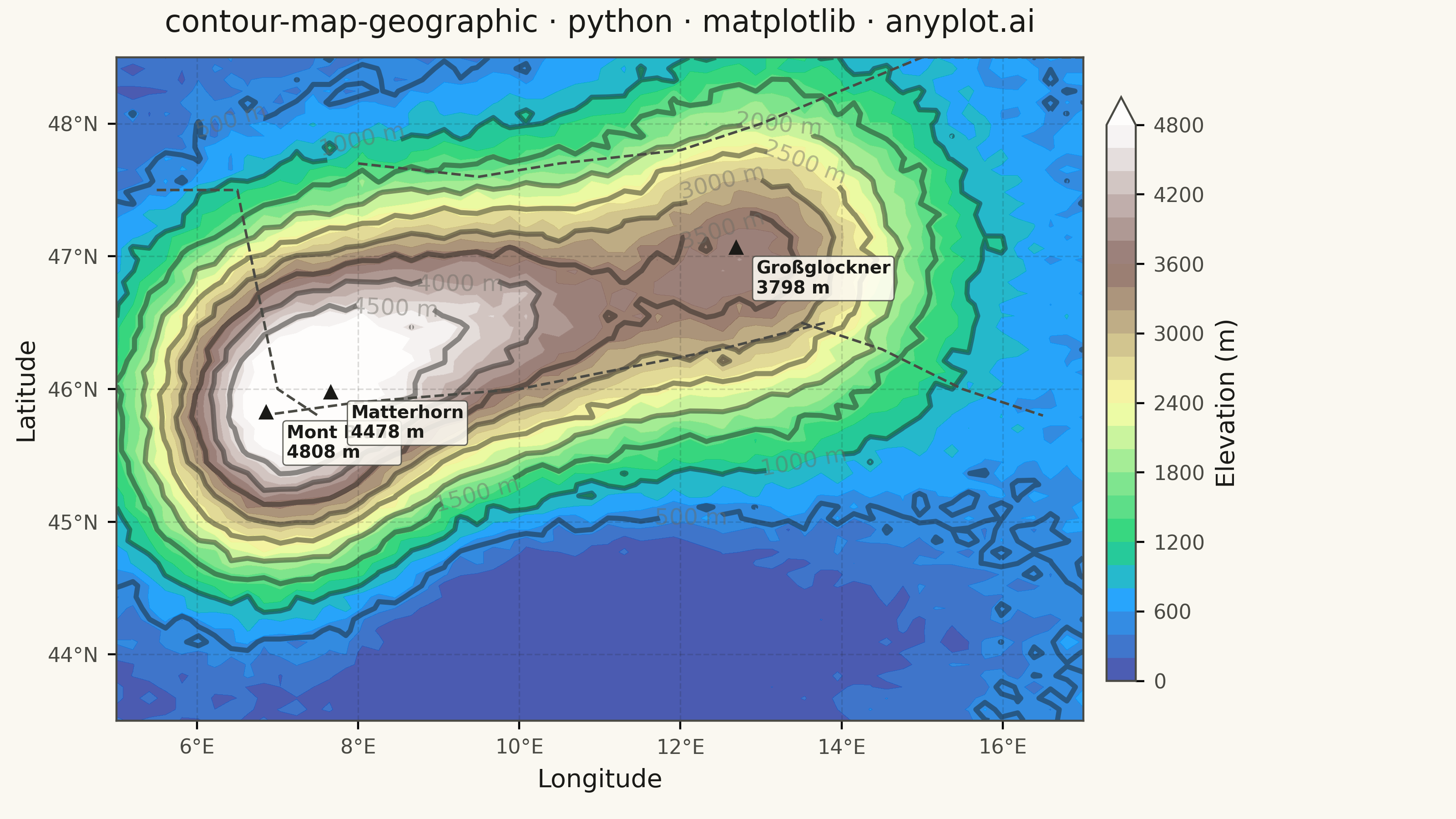
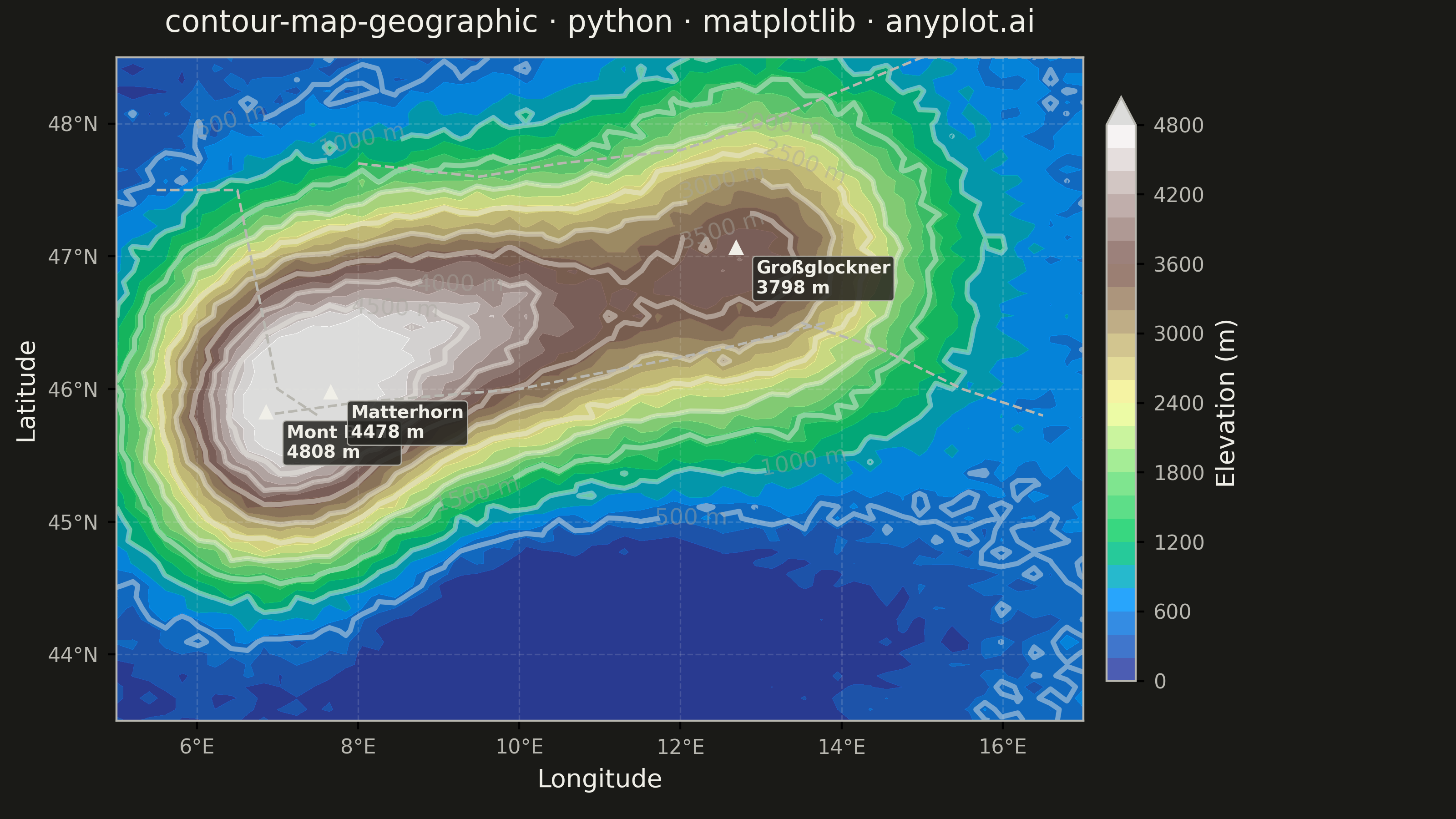
Contour Lines on Geographic Map — Matplotlib

A contour map overlays isolines (lines of equal value) onto a geographic basemap, visualizing continuous spatial data such as elevation, temperature, or atmospheric pressure across real-world coordinates. Unlike basic contour plots that use abstract x/y coordinates, this plot anchors contours to latitude/longitude positions with geographic context like coastlines, borders, or terrain. It combines the precision of isoline visualization with spatial awareness, making it ideal for meteorological, topographic, and environmental applications.

Contour Lines on Geographic Map rendered with Matplotlib

Python source (Matplotlib)

""" anyplot.ai
contour-map-geographic: Contour Lines on Geographic Map
Library: matplotlib 3.10.9 | Python 3.13.13
Quality: 90/100 | Updated: 2026-05-20
"""

import os

import matplotlib.pyplot as plt
import numpy as np


# Theme tokens
THEME = os.getenv("ANYPLOT_THEME", "light")
PAGE_BG = "#FAF8F1" if THEME == "light" else "#1A1A17"
ELEVATED_BG = "#FFFDF6" if THEME == "light" else "#242420"
INK = "#1A1A17" if THEME == "light" else "#F0EFE8"
INK_SOFT = "#4A4A44" if THEME == "light" else "#B8B7B0"
INK_MUTED = "#6B6A63" if THEME == "light" else "#A8A79F"

# Data: Synthetic elevation data over European Alps
np.random.seed(42)

lon_min, lon_max = 5.0, 17.0
lat_min, lat_max = 43.5, 48.5

n_points = 60
lons = np.linspace(lon_min, lon_max, n_points)
lats = np.linspace(lat_min, lat_max, n_points)
lon_grid, lat_grid = np.meshgrid(lons, lats)

# Base undulating terrain
elevation = 400 + 200 * np.sin(np.radians(lon_grid) * 15) * np.cos(np.radians(lat_grid) * 12)

# Western Alps: Mont Blanc massif (~4808 m peak)
elevation += 4400 * np.exp(-((lon_grid - 7.0) ** 2) / 3) * np.exp(-((lat_grid - 45.8) ** 2) / 1.5)

# Central Swiss Alps
elevation += 3600 * np.exp(-((lon_grid - 9.5) ** 2) / 5) * np.exp(-((lat_grid - 46.5) ** 2) / 1.2)

# Austrian Tyrol / Hohe Tauern (Großglockner ~3798 m)
elevation += 3000 * np.exp(-((lon_grid - 13.0) ** 2) / 4) * np.exp(-((lat_grid - 47.0) ** 2) / 1.5)

# Po Valley lowlands (Italian side — low elevation)
elevation -= 700 * np.exp(-((lon_grid - 11.0) ** 2) / 20) * np.exp(-((lat_grid - 44.2) ** 2) / 0.8)

# Add noise for realism
elevation += np.random.normal(0, 80, elevation.shape)
elevation = np.clip(elevation, 0, None)

# Simplified country border lines
borders = [
    {"lons": [5.5, 6.5, 7.0, 7.5], "lats": [47.5, 47.5, 46.0, 45.8]},
    {"lons": [6.8, 8.0, 10.0, 12.5, 13.8], "lats": [45.8, 45.9, 46.0, 46.3, 46.5]},
    {"lons": [8.0, 9.5, 10.5, 12.0, 13.0, 15.0, 17.0], "lats": [47.7, 47.6, 47.7, 47.8, 48.0, 48.5, 48.5]},
    {"lons": [13.5, 14.5, 15.5, 16.5], "lats": [46.5, 46.3, 46.0, 45.8]},
]

# Notable peaks to annotate
peaks = [
    {"name": "Mont Blanc\n4808 m", "lon": 6.86, "lat": 45.83},
    {"name": "Matterhorn\n4478 m", "lon": 7.66, "lat": 45.98},
    {"name": "Großglockner\n3798 m", "lon": 12.69, "lat": 47.07},
]

# Plot
fig, ax = plt.subplots(figsize=(8, 4.5), dpi=400, facecolor=PAGE_BG)
ax.set_facecolor(PAGE_BG)

# Filled contours using terrain colormap
levels = np.arange(0, 5000, 200)
filled = ax.contourf(lon_grid, lat_grid, elevation, levels=levels, cmap="terrain", alpha=0.85, extend="max")

# Contour lines every 500 m — heavier weight for high-res visibility
line_levels = np.arange(500, 5000, 500)
contour_lines = ax.contour(lon_grid, lat_grid, elevation, levels=line_levels, colors=INK, linewidths=2.0, alpha=0.45)
ax.clabel(contour_lines, inline=True, fontsize=9, fmt="%d m", colors=INK_MUTED)

# Country border lines
for border in borders:
    ax.plot(border["lons"], border["lats"], color=INK_SOFT, linewidth=1.0, linestyle="--", zorder=4)

# Peak markers and annotations — focal point emphasis
for peak in peaks:
    ax.plot(peak["lon"], peak["lat"], marker="^", markersize=6, color=INK, zorder=6, markeredgewidth=0)
    ax.annotate(
        peak["name"],
        xy=(peak["lon"], peak["lat"]),
        xytext=(peak["lon"] + 0.25, peak["lat"] - 0.35),
        fontsize=7,
        color=INK,
        fontweight="bold",
        bbox={
            "facecolor": ELEVATED_BG,
            "edgecolor": INK_SOFT,
            "alpha": 0.85,
            "boxstyle": "round,pad=0.2",
            "linewidth": 0.5,
        },
        zorder=7,
    )

# Colorbar — idiomatic fig.colorbar
cbar = fig.colorbar(filled, ax=ax, orientation="vertical", pad=0.02, shrink=0.88)
cbar.set_label("Elevation (m)", fontsize=10, color=INK)
cbar.ax.tick_params(labelsize=8, labelcolor=INK_SOFT)
cbar.outline.set_edgecolor(INK_SOFT)

# Axis limits and tick formatting
ax.set_xlim(lon_min, lon_max)
ax.set_ylim(lat_min, lat_max)

lon_ticks = np.arange(6, 17, 2)
ax.set_xticks(lon_ticks)
ax.set_xticklabels([f"{int(x)}°E" for x in lon_ticks])

lat_ticks = np.arange(44, 49, 1)
ax.set_yticks(lat_ticks)
ax.set_yticklabels([f"{int(y)}°N" for y in lat_ticks])

ax.tick_params(axis="both", labelsize=8, labelcolor=INK_SOFT)

# Axis labels
ax.set_xlabel("Longitude", fontsize=10, color=INK)
ax.set_ylabel("Latitude", fontsize=10, color=INK)

# Title
ax.set_title(
    "contour-map-geographic · python · matplotlib · anyplot.ai", fontsize=12, fontweight="medium", color=INK, pad=10
)

# Spines — keep all four as map border, color-adapt them
for spine in ax.spines.values():
    spine.set_color(INK_SOFT)

# Subtle grid
ax.grid(True, alpha=0.15, linewidth=0.6, color=INK, linestyle="--", zorder=1)

fig.subplots_adjust(left=0.08, right=0.88, top=0.93, bottom=0.12)

plt.savefig(f"plot-{THEME}.png", dpi=400, facecolor=PAGE_BG)
plt.close()

Part of Contour Lines on Geographic Map on anyplot.ai.

Contour Lines on Geographic Map — Matplotlib

Python source (Matplotlib)

Other implementations