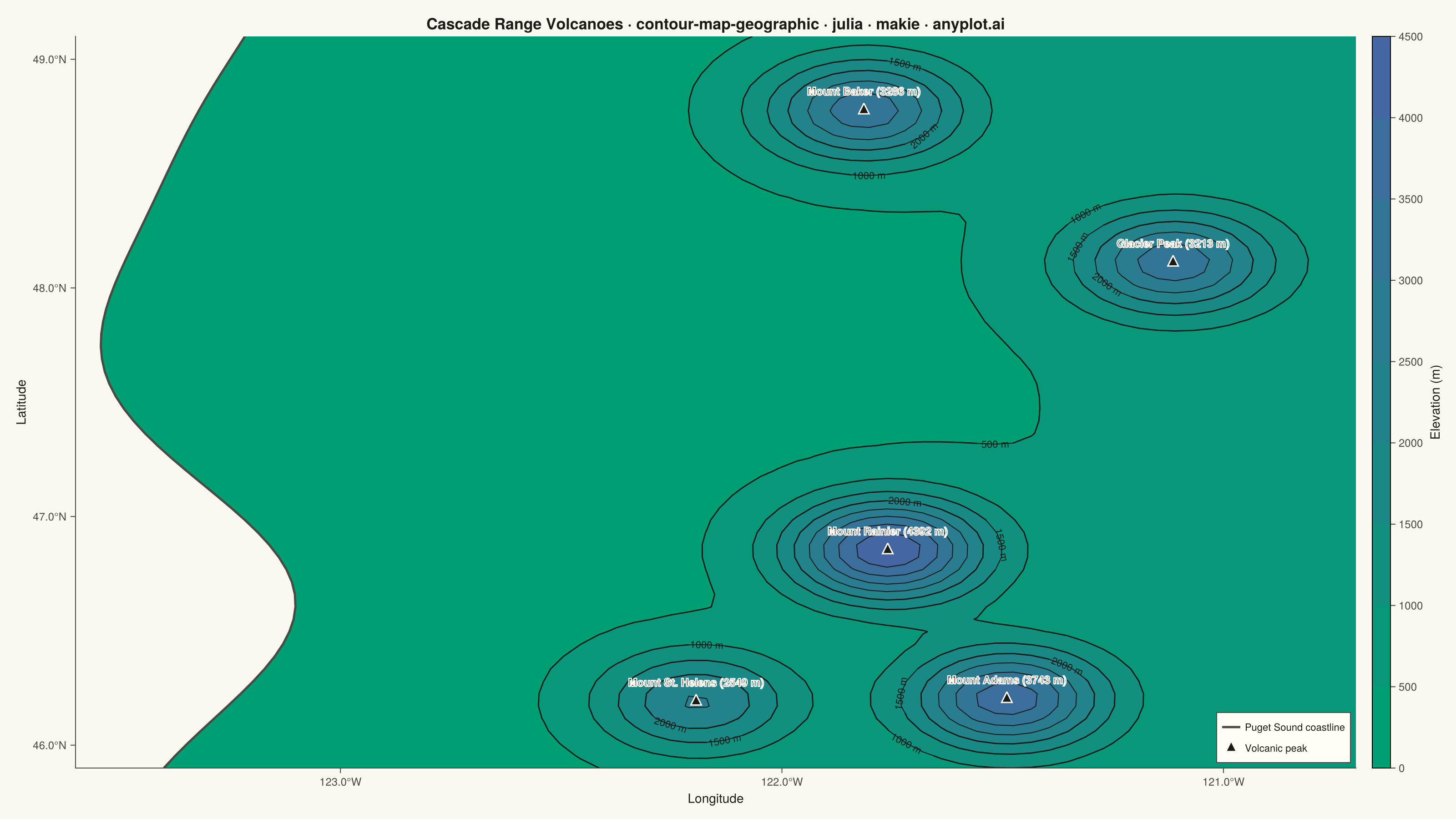
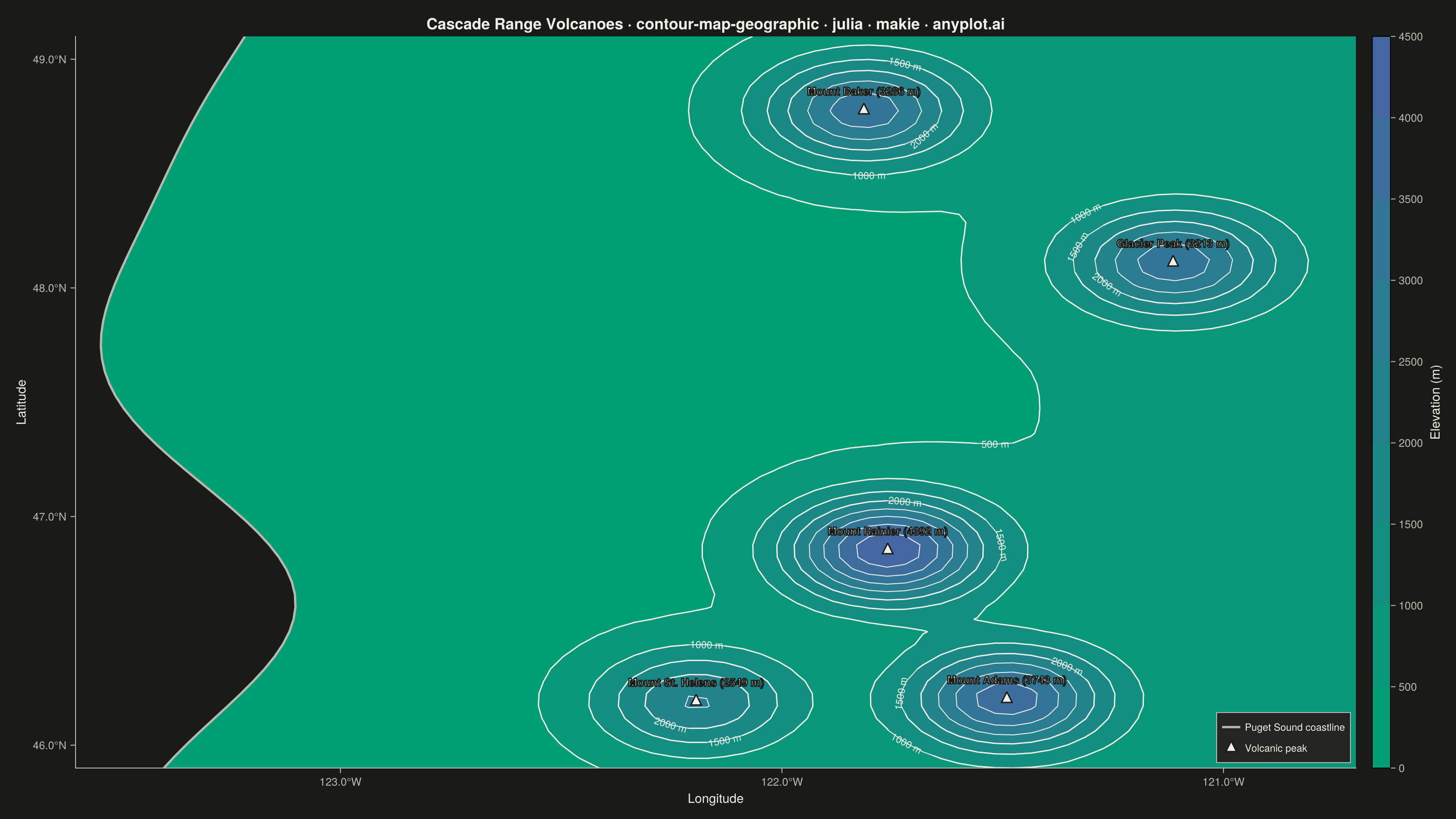
The same plot in 14 other libraries — Python: Altair, Bokeh, lets-plot, Matplotlib, Plotly, plotnine, Pygal, Seaborn; R: ggplot2; JavaScript: Chart.js, D3.js, Apache ECharts, Highcharts, MUI X Charts. Compare all 15 side by side: Contour Lines on Geographic Map in Python, R, Julia and JavaScript.
A contour map overlays isolines (lines of equal value) onto a geographic basemap, visualizing continuous spatial data such as elevation, temperature, or atmospheric pressure across real-world coordinates. Unlike basic contour plots that use abstract x/y coordinates, this plot anchors contours to latitude/longitude positions with geographic context like coastlines, borders, or terrain. It combines the precision of isoline visualization with spatial awareness, making it ideal for meteorological, topographic, and environmental applications.
# anyplot.ai
# contour-map-geographic: Contour Lines on Geographic Map
# Library: makie 0.21.9 | Julia 1.11.9
# Quality: 93/100 | Created: 2026-09-01

using CairoMakie
using Colors
using Random

Random.seed!(42)

# Theme tokens
const THEME       = get(ENV, "ANYPLOT_THEME", "light")
const PAGE_BG     = THEME == "light" ? colorant"#FAF8F1" : colorant"#1A1A17"
const ELEVATED_BG = THEME == "light" ? colorant"#FFFDF6" : colorant"#242420"
const INK         = THEME == "light" ? colorant"#1A1A17" : colorant"#F0EFE8"
const INK_SOFT    = THEME == "light" ? colorant"#4A4A44" : colorant"#B8B7B0"
const ANYPLOT_SEQ = cgrad([colorant"#009E73", colorant"#4467A3"])

# Data — synthetic elevation grid over the Cascade Range stratovolcanoes (Washington, USA)
const PEAKS = [
    (name = "Mount Baker",      lat = 48.7768, lon = -121.8144, elev = 3286.0),
    (name = "Glacier Peak",     lat = 48.1112, lon = -121.1141, elev = 3213.0),
    (name = "Mount Rainier",    lat = 46.8529, lon = -121.7604, elev = 4392.0),
    (name = "Mount Adams",      lat = 46.2024, lon = -121.4906, elev = 3743.0),
    (name = "Mount St. Helens", lat = 46.1912, lon = -122.1944, elev = 2549.0),
]

const lon = range(-123.6, -120.7; length = 72)
const lat = range(45.9, 49.1; length = 60)

# Rolling foothill baseline (west→east) plus a Gaussian bump per named summit
const z = [
    250.0 + 350.0 * clamp((lo + 123.2) / 2.5, 0.0, 1.0) +
    sum((p.elev - 380.0) * exp(-(((lo - p.lon) / 0.22)^2 + ((la - p.lat) / 0.22)^2)) for p in PEAKS)
    for lo in lon, la in lat
]

const LEVELS       = collect(0.0:500.0:4500.0)
const LABEL_LEVELS = collect(0.0:500.0:2000.0)  # index contours — the tight rings near each
                                                 # summit stay unlabeled since the peak marker
                                                 # already states the exact elevation there

# Puget Sound coastline: a wavy west boundary marking land vs. water
const lat_vec   = collect(lat)
const coast_lon = @. -123.35 + 0.20 * sin(2.3 * (lat_vec - 45.9)) - 0.05 * cos(4.1 * (lat_vec - 45.9))

# Plot
fig = Figure(
    size            = (1600, 900),
    fontsize        = 14,
    backgroundcolor = PAGE_BG,
)

ax = Axis(
    fig[1, 1];
    title              = "Cascade Range Volcanoes · contour-map-geographic · julia · makie · anyplot.ai",
    titlesize          = 17,
    titlecolor         = INK,
    xlabel             = "Longitude",
    ylabel             = "Latitude",
    xlabelsize         = 14,
    ylabelsize         = 14,
    xlabelcolor        = INK,
    ylabelcolor        = INK,
    xticklabelsize     = 12,
    yticklabelsize     = 12,
    xticklabelcolor    = INK_SOFT,
    yticklabelcolor    = INK_SOFT,
    xtickcolor         = INK_SOFT,
    ytickcolor         = INK_SOFT,
    xtickformat        = vs -> ["$(round(abs(v), digits = 1))°W" for v in vs],
    ytickformat        = vs -> ["$(round(v, digits = 1))°N" for v in vs],
    backgroundcolor    = PAGE_BG,
    topspinevisible    = false,
    rightspinevisible  = false,
    leftspinecolor     = INK_SOFT,
    bottomspinecolor   = INK_SOFT,
    xgridcolor         = RGBAf(INK.r, INK.g, INK.b, 0.12),
    ygridcolor         = RGBAf(INK.r, INK.g, INK.b, 0.12),
    limits             = (minimum(lon), maximum(lon), minimum(lat), maximum(lat)),
)

# Filled elevation contours
cf = contourf!(ax, lon, lat, z; levels = LEVELS, colormap = ANYPLOT_SEQ)

# Contour lines at every 500 m
contour!(ax, lon, lat, z; levels = LEVELS, color = INK, linewidth = 1.0)

# Index contours (every 500 m up to 2000 m) carry the value labels — the
# tighter rings closer to each summit are left unlabeled to avoid crowding
# the peak-name labels below
contour!(ax, lon, lat, z;
    levels         = LABEL_LEVELS,
    color          = INK,
    linewidth      = 1.4,
    labels         = true,
    labelsize      = 11,
    labelcolor     = INK,
    labelformatter = level -> "$(Int(round(level))) m",
)

# Mask the water west of the coastline, then stroke the shoreline itself
west_edge  = minimum(lon) - 0.3
water_poly = vcat(
    [Point2f(coast_lon[i], lat_vec[i]) for i in eachindex(lat_vec)],
    [Point2f(west_edge, lat_vec[i]) for i in reverse(eachindex(lat_vec))],
)
poly!(ax, water_poly; color = PAGE_BG, strokewidth = 0)
lines!(ax, coast_lon, lat_vec; color = INK_SOFT, linewidth = 2.5, label = "Puget Sound coastline")

# Volcanic summits, labeled with elevation
scatter!(ax, [p.lon for p in PEAKS], [p.lat for p in PEAKS];
    marker      = :utriangle,
    markersize  = 16,
    color       = INK,
    strokewidth = 1.5,
    strokecolor = PAGE_BG,
    label       = "Volcanic peak",
)
for p in PEAKS
    text!(ax, p.lon, p.lat;
        text        = "$(p.name) ($(Int(round(p.elev))) m)",
        fontsize    = 12,
        font        = :bold,
        color       = INK,
        strokecolor = PAGE_BG,
        strokewidth = 1.3,
        align       = (:center, :bottom),
        offset      = (0, 14),
    )
end

axislegend(ax;
    position        = :rb,
    backgroundcolor = ELEVATED_BG,
    labelcolor      = INK,
    framecolor      = INK_SOFT,
    labelsize       = 11,
)

Colorbar(fig[1, 2], cf;
    label          = "Elevation (m)",
    labelcolor     = INK,
    labelsize      = 14,
    tickcolor      = INK_SOFT,
    ticklabelcolor = INK_SOFT,
    ticklabelsize  = 12,
    ticks          = LEVELS,
    width          = 20,
)

# Save
save("plot-$(THEME).png", fig; px_per_unit = 2)
Runnable source as JSON, for any HTTP client: https://api.anyplot.ai/specs/contour-map-geographic/makie/code. Any spec id and library id listed in llms-full.txt fit the same URL shape; every URL below is complete and callable.
{
  "spec_id": "contour-map-geographic",
  "language": "julia",
  "library": "makie",
  "page": "https://anyplot.ai/contour-map-geographic/julia/makie",
  "hub": "https://anyplot.ai/contour-map-geographic",
  "code_json": "https://api.anyplot.ai/specs/contour-map-geographic/makie/code",
  "spec_json": "https://api.anyplot.ai/specs/contour-map-geographic",
  "render_light_png": "https://storage.googleapis.com/anyplot-images/plots/contour-map-geographic/julia/makie/plot-light.png",
  "render_dark_png": "https://storage.googleapis.com/anyplot-images/plots/contour-map-geographic/julia/makie/plot-dark.png",
  "quality_score": 93.0,
  "license": "MIT",
  "guide": "https://anyplot.ai/llms.txt"
}
Part of Contour Lines on Geographic Map on anyplot.ai.