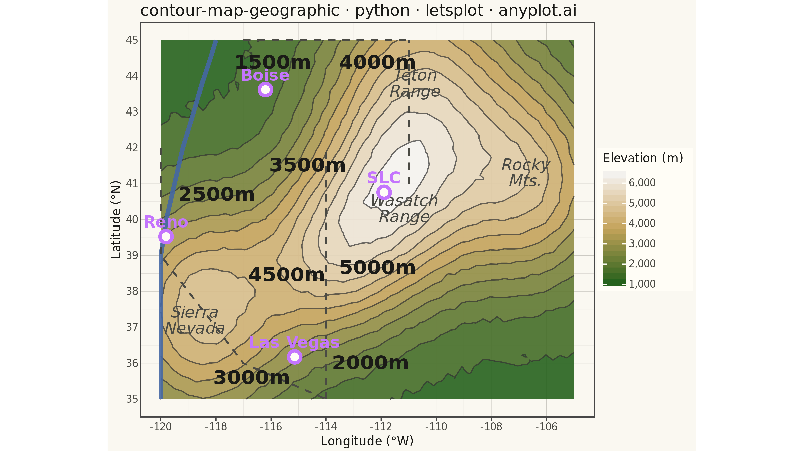
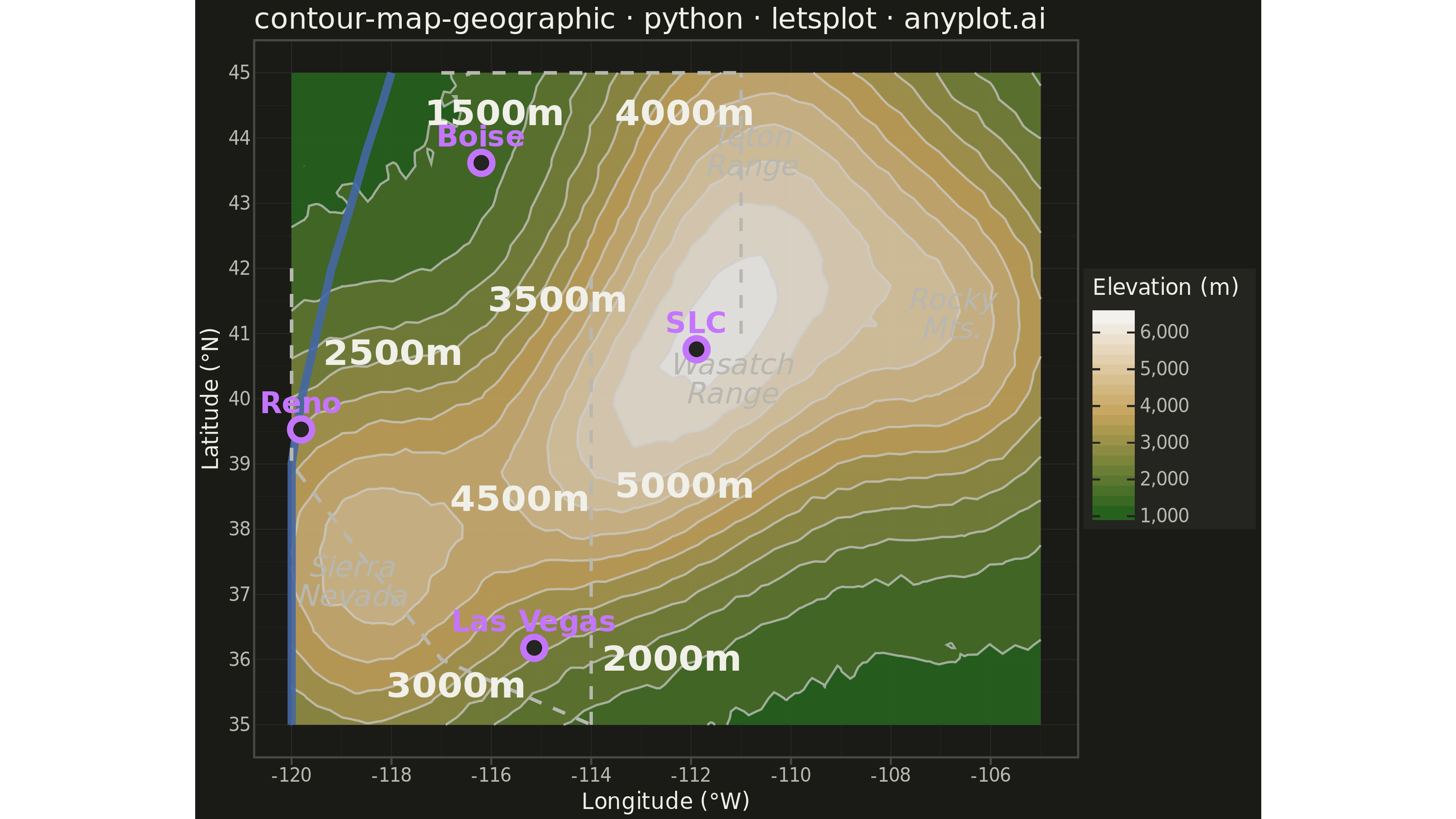
A contour map overlays isolines (lines of equal value) onto a geographic basemap, visualizing continuous spatial data such as elevation, temperature, or atmospheric pressure across real-world coordinates. Unlike basic contour plots that use abstract x/y coordinates, this plot anchors contours to latitude/longitude positions with geographic context like coastlines, borders, or terrain. It combines the precision of isoline visualization with spatial awareness, making it ideal for meteorological, topographic, and environmental applications.
""" anyplot.ai
contour-map-geographic: Contour Lines on Geographic Map
Library: letsplot 4.10.1 | Python 3.13.13
Quality: 86/100 | Updated: 2026-05-20
"""

import os

import numpy as np
import pandas as pd
from lets_plot import (
    LetsPlot,
    aes,
    coord_fixed,
    element_blank,
    element_line,
    element_rect,
    element_text,
    geom_contour,
    geom_contourf,
    geom_path,
    geom_point,
    geom_text,
    ggplot,
    ggsize,
    labs,
    scale_fill_gradient2,
    theme,
)
from lets_plot.export import ggsave


LetsPlot.setup_html()

# Theme tokens
THEME = os.getenv("ANYPLOT_THEME", "light")
PAGE_BG = "#FAF8F1" if THEME == "light" else "#1A1A17"
ELEVATED_BG = "#FFFDF6" if THEME == "light" else "#242420"
INK = "#1A1A17" if THEME == "light" else "#F0EFE8"
INK_SOFT = "#4A4A44" if THEME == "light" else "#B8B7B0"
CONTOUR_COLOR = "#333333" if THEME == "light" else "#CCCCCC"
LABEL_COLOR = "#1A1A17" if THEME == "light" else "#F0EFE8"
COAST_COLOR = "#4467A3"  # Okabe-Ito blue — works on both themes
GRID_MAJOR = "#CCCAC3" if THEME == "light" else "#2E2E2B"
GRID_MINOR = "#E0DDD7" if THEME == "light" else "#252522"
CITY_COLOR = "#C475FD"  # Okabe-Ito vermillion — reference cities
ANNO_BG = "#FFFDF6" if THEME == "light" else "#242420"

# Data — synthetic elevation for Western US mountain region
np.random.seed(42)

lat_range = np.linspace(35, 45, 50)
lon_range = np.linspace(-120, -105, 60)
lon_grid, lat_grid = np.meshgrid(lon_range, lat_range)

elevation = np.zeros_like(lat_grid)

peaks = [
    (40.5, -111.5, 2800, 2.0),  # Wasatch Range near Salt Lake City
    (39.0, -114.0, 2600, 1.8),  # Nevada peak (Great Basin)
    (43.5, -110.5, 3200, 2.5),  # Tetons area
    (37.5, -118.5, 3500, 2.2),  # Sierra Nevada
    (41.0, -106.5, 2900, 2.0),  # Rocky Mountains
]

for peak_lat, peak_lon, peak_height, spread in peaks:
    distance = np.sqrt((lat_grid - peak_lat) ** 2 + (lon_grid - peak_lon) ** 2)
    elevation += peak_height * np.exp(-(distance**2) / (2 * spread**2))

elevation += 1200 + np.random.randn(*elevation.shape) * 30

df = pd.DataFrame({"lon": lon_grid.flatten(), "lat": lat_grid.flatten(), "elevation": elevation.flatten()})

elev_min = int(np.floor(elevation.min() / 500) * 500)
elev_max = int(np.ceil(elevation.max() / 500) * 500)
elev_mid = (elev_min + elev_max) / 2

# Contour labels at 500m intervals for better readability
contour_levels = [1500, 2000, 2500, 3000, 3500, 4000, 4500, 5000]

label_data = []
used_positions = []

for level in contour_levels:
    candidates = df[
        (abs(df["elevation"] - level) < 80)
        & (df["lon"] > lon_range[0] + 2.0)  # 2° left buffer to prevent text clipping
        & (df["lon"] < lon_range[-1] - 7.0)  # 7° right buffer to avoid panel clipping
        & (df["lat"] > lat_range[0] + 0.5)
        & (df["lat"] < lat_range[-1] - 0.5)
    ].copy()
    if len(candidates) == 0:
        continue

    best_candidate = None
    best_dist = 0

    for _, row in candidates.iterrows():
        min_dist = float("inf")
        for used_lon, used_lat in used_positions:
            dist = np.sqrt((row["lon"] - used_lon) ** 2 + (row["lat"] - used_lat) ** 2)
            min_dist = min(min_dist, dist)

        if len(used_positions) == 0 or min_dist > best_dist:
            best_dist = min_dist
            best_candidate = row

    if best_candidate is not None and (len(used_positions) == 0 or best_dist > 1.5):
        label_data.append({"lon": best_candidate["lon"], "lat": best_candidate["lat"], "label": f"{int(level)}m"})
        used_positions.append((best_candidate["lon"], best_candidate["lat"]))

label_df = pd.DataFrame(label_data) if label_data else pd.DataFrame({"lon": [], "lat": [], "label": []})

# Geographic features — Pacific coastline (more detail for realism)
coast_df = pd.DataFrame(
    {
        "lon": [-120, -120, -120, -120, -119.8, -119.5, -119.2, -118.8, -118.5, -118.2, -118],
        "lat": [35, 36, 37.5, 39, 40, 41, 42, 43, 43.8, 44.5, 45],
    }
)

# State border segments (CA/NV, NV/UT, ID/UT, WY/MT/ID borders)
border_segments = [
    {"lon": [-120, -120, -117, -114], "lat": [42, 39, 36, 35]},
    {"lon": [-114, -114], "lat": [35, 42]},
    {"lon": [-111, -111], "lat": [41, 45]},
    {"lon": [-117, -111], "lat": [45, 45]},
]
border_dfs = [pd.DataFrame(seg) for seg in border_segments]

# Mountain range name annotations — storytelling layer
range_labels = pd.DataFrame(
    {
        "lon": [-118.8, -111.2, -110.8, -106.8],
        "lat": [37.2, 40.3, 43.8, 41.3],
        "label": ["Sierra\nNevada", "Wasatch\nRange", "Teton\nRange", "Rocky\nMts."],
    }
)

# Reference cities inside the plot bounds for geographic context
cities = pd.DataFrame(
    {
        "lon": [-119.81, -115.14, -111.89, -116.20],
        "lat": [39.53, 36.18, 40.76, 43.62],
        "label": ["Reno", "Las Vegas", "SLC", "Boise"],
    }
)

# Build plot
plot = (
    ggplot(df, aes(x="lon", y="lat", z="elevation"))
    + geom_contourf(aes(fill="..level.."), bins=12, alpha=0.9)
    + geom_contour(color=CONTOUR_COLOR, size=0.5, bins=12, alpha=0.7)
    + scale_fill_gradient2(
        low="#1a5e1a",
        mid="#c4a35a",
        high="#f5f5f5",
        midpoint=elev_mid,
        limits=[elev_min, elev_max],
        name="Elevation (m)",
    )
    + geom_path(data=coast_df, mapping=aes(x="lon", y="lat"), color=COAST_COLOR, size=2.0, alpha=0.9, inherit_aes=False)
)

for border_df in border_dfs:
    plot = plot + geom_path(
        data=border_df, mapping=aes(x="lon", y="lat"), color=INK_SOFT, size=0.8, linetype="dashed", inherit_aes=False
    )

if len(label_df) > 0:
    plot = plot + geom_text(
        data=label_df,
        mapping=aes(x="lon", y="lat", label="label"),
        color=LABEL_COLOR,
        size=10,  # increased from 9 for mobile legibility
        fontface="bold",
        inherit_aes=False,
    )

# Mountain range annotations — italic, slightly smaller for hierarchy
plot = plot + geom_text(
    data=range_labels,
    mapping=aes(x="lon", y="lat", label="label"),
    color=INK_SOFT,
    size=8,
    fontface="italic",
    inherit_aes=False,
)

# City reference markers + labels
plot = plot + geom_point(
    data=cities,
    mapping=aes(x="lon", y="lat"),
    color=CITY_COLOR,
    size=4,
    shape=21,
    fill=ANNO_BG,
    stroke=1.5,
    inherit_aes=False,
)
plot = plot + geom_text(
    data=cities,
    mapping=aes(x="lon", y="lat", label="label"),
    color=CITY_COLOR,
    size=8,
    nudge_y=0.4,
    fontface="bold",
    inherit_aes=False,
)

# Theme-adaptive chrome — no heavy base theme; fully custom for map-style clarity
anyplot_theme = theme(
    plot_background=element_rect(fill=PAGE_BG, color=PAGE_BG),
    panel_background=element_rect(fill=PAGE_BG),
    panel_border=element_blank(),  # geographic maps conventionally use no heavy frame
    panel_grid_major=element_line(color=GRID_MAJOR, size=0.3),
    panel_grid_minor=element_line(color=GRID_MINOR, size=0.2),
    axis_title=element_text(color=INK, size=12),
    axis_text=element_text(color=INK_SOFT, size=10),
    axis_line=element_line(color=INK_SOFT, size=0.5),
    plot_title=element_text(color=INK, size=16),
    legend_background=element_rect(fill=ELEVATED_BG, color=INK_SOFT),
    legend_text=element_text(color=INK_SOFT, size=10),
    legend_title=element_text(color=INK, size=12),
    legend_position="right",
)

# Geographic aspect ratio correction for ~40°N latitude
geo_ratio = 1.0 / np.cos(np.radians(40.0))

plot = (
    plot
    + labs(title="contour-map-geographic · python · letsplot · anyplot.ai", x="Longitude (°W)", y="Latitude (°N)")
    + anyplot_theme
    + ggsize(800, 450)
    + coord_fixed(ratio=geo_ratio)
)

# Save — theme-suffixed filenames
ggsave(plot, f"plot-{THEME}.png", path=".", scale=4)
ggsave(plot, f"plot-{THEME}.html", path=".")
Runnable source as JSON, for any HTTP client: https://api.anyplot.ai/specs/contour-map-geographic/letsplot/code. Any spec id and library id listed in llms-full.txt fit the same URL shape; every URL below is complete and callable.
{
  "spec_id": "contour-map-geographic",
  "language": "python",
  "library": "letsplot",
  "page": "https://anyplot.ai/contour-map-geographic/python/letsplot",
  "hub": "https://anyplot.ai/contour-map-geographic",
  "code_json": "https://api.anyplot.ai/specs/contour-map-geographic/letsplot/code",
  "spec_json": "https://api.anyplot.ai/specs/contour-map-geographic",
  "render_light_png": "https://storage.googleapis.com/anyplot-images/plots/contour-map-geographic/python/letsplot/plot-light.png",
  "render_dark_png": "https://storage.googleapis.com/anyplot-images/plots/contour-map-geographic/python/letsplot/plot-dark.png",
  "interactive_light_html": "https://storage.googleapis.com/anyplot-images/plots/contour-map-geographic/python/letsplot/plot-light.html",
  "interactive_dark_html": "https://storage.googleapis.com/anyplot-images/plots/contour-map-geographic/python/letsplot/plot-dark.html",
  "quality_score": 86.0,
  "license": "MIT",
  "guide": "https://anyplot.ai/llms.txt"
}
Part of Contour Lines on Geographic Map on anyplot.ai.