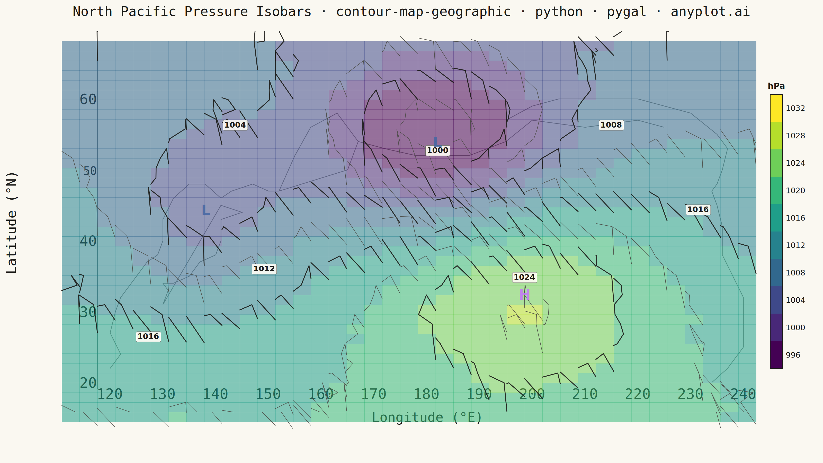
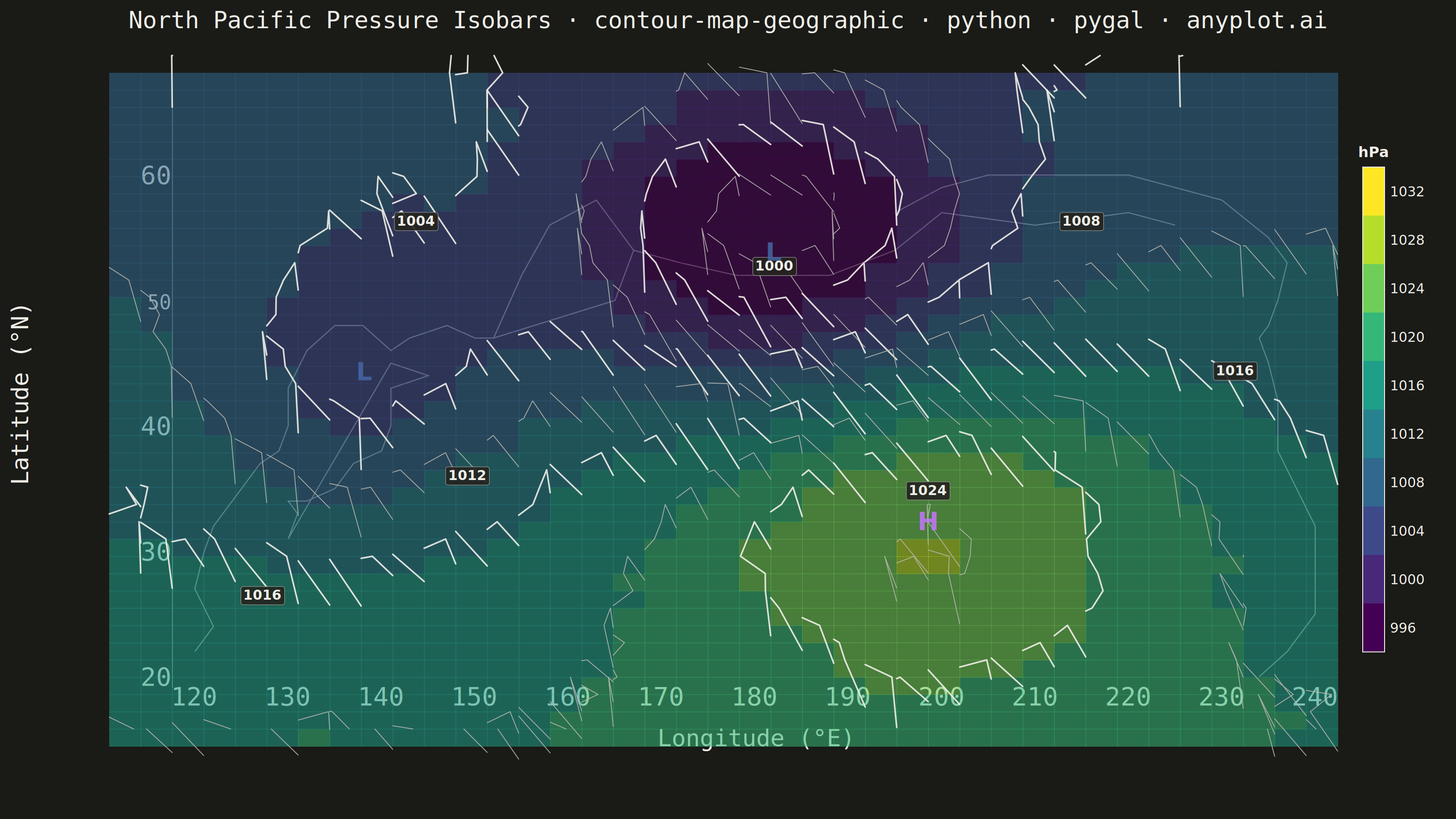
A contour map overlays isolines (lines of equal value) onto a geographic basemap, visualizing continuous spatial data such as elevation, temperature, or atmospheric pressure across real-world coordinates. Unlike basic contour plots that use abstract x/y coordinates, this plot anchors contours to latitude/longitude positions with geographic context like coastlines, borders, or terrain. It combines the precision of isoline visualization with spatial awareness, making it ideal for meteorological, topographic, and environmental applications.
""" anyplot.ai
contour-map-geographic: Contour Lines on Geographic Map
Library: pygal 3.1.0 | Python 3.13.13
Quality: 87/100 | Updated: 2026-05-20
"""

import os
import sys
from pathlib import Path


sys.path = [p for p in sys.path if p != str(Path(__file__).parent)]

import cairosvg
import matplotlib.cm as mpl_cm
import matplotlib.colors as mpl_colors
import numpy as np
import pygal as pygal_lib
from pygal.style import Style


THEME = os.getenv("ANYPLOT_THEME", "light")
PAGE_BG = "#FAF8F1" if THEME == "light" else "#1A1A17"
ELEVATED_BG = "#FFFDF6" if THEME == "light" else "#242420"
INK = "#1A1A17" if THEME == "light" else "#F0EFE8"
INK_SOFT = "#4A4A44" if THEME == "light" else "#B8B7B0"
INK_MUTED = "#6B6A63" if THEME == "light" else "#A8A79F"

# Data — North Pacific sea-level pressure field (hPa)
np.random.seed(42)

lon_min, lon_max = 120, 240  # 120°E to 120°W
lat_min, lat_max = 20, 65

n_grid = 40
lon_grid = np.linspace(lon_min, lon_max, n_grid)
lat_grid = np.linspace(lat_min, lat_max, n_grid)
LON, LAT = np.meshgrid(lon_grid, lat_grid)

# Background pressure gradient (higher in subtropics, lower at poles)
pressure_base = 1020 - (LAT - lat_min) * 0.25

# North Pacific High (subtropical high pressure ridge)
hp_lon, hp_lat = 200, 35
dist_hp = np.sqrt(((LON - hp_lon) / 25) ** 2 + ((LAT - hp_lat) / 12) ** 2)
pressure_base += 12 * np.exp(-(dist_hp**2))

# Aleutian Low (subpolar low pressure center)
al_lon, al_lat = 185, 53
dist_al = np.sqrt(((LON - al_lon) / 20) ** 2 + ((LAT - al_lat) / 10) ** 2)
pressure_base -= 18 * np.exp(-(dist_al**2))

# Secondary low off Asian coast
al2_lon, al2_lat = 145, 45
dist_al2 = np.sqrt(((LON - al2_lon) / 15) ** 2 + ((LAT - al2_lat) / 10) ** 2)
pressure_base -= 8 * np.exp(-(dist_al2**2))

PRESSURE = pressure_base + np.random.normal(0, 0.3, pressure_base.shape)

# Isobar levels every 4 hPa
contour_levels = np.arange(996, 1033, 4)

# Simplified coastlines: North Pacific rim (lon, lat)
coastlines = [
    # Japan main islands
    [
        (130, 31),
        (131, 33),
        (130, 34),
        (132, 34),
        (135, 35),
        (137, 37),
        (140, 38),
        (141, 40),
        (141, 43),
        (145, 44),
        (141, 45),
        (130, 31),
    ],
    # Kamchatka + Kuril arc
    [(152, 47), (155, 52), (158, 56), (163, 58), (167, 54), (165, 50), (152, 47)],
    # Aleutian Islands (simplified)
    [(167, 54), (172, 53), (178, 52), (188, 52), (195, 54), (200, 57), (210, 56), (220, 57), (225, 56)],
    # Alaska
    [(195, 57), (200, 59), (205, 60), (210, 60), (215, 60), (220, 60), (225, 59), (230, 58), (235, 55), (237, 53)],
    # North American west coast
    [
        (237, 53),
        (236, 50),
        (235, 48),
        (234, 47),
        (235, 45),
        (236, 42),
        (236, 38),
        (238, 35),
        (240, 32),
        (240, 25),
        (237, 22),
        (234, 20),
    ],
    # Asian mainland coast (rough)
    [
        (120, 22),
        (122, 24),
        (120, 27),
        (121, 30),
        (122, 32),
        (124, 34),
        (127, 37),
        (129, 38),
        (130, 40),
        (130, 43),
        (132, 46),
        (135, 48),
        (138, 48),
        (141, 46),
        (143, 47),
        (147, 48),
        (150, 47),
        (152, 47),
    ],
]

# Pressure colormap: viridis sequential (perceptually uniform, style-guide compliant)
p_min_cb, p_max_cb = 996, 1032
n_colors = 10
pressure_colors = [mpl_colors.to_hex(mpl_cm.viridis(i / (n_colors - 1))) for i in range(n_colors)]

custom_style = Style(
    background=PAGE_BG,
    plot_background=PAGE_BG,
    foreground=INK,
    foreground_strong=INK,
    foreground_subtle=INK_MUTED,
    guide_stroke_color="rgba(128,128,128,0.15)",
    guide_stroke_dasharray="",
    colors=(INK_MUTED,) * (len(coastlines) + 1),
    title_font_size=52,
    label_font_size=56,
    major_label_font_size=44,
    legend_font_size=44,
    value_font_size=36,
    stroke_width=2.5,
)

chart = pygal_lib.XY(
    width=3200,
    height=1800,
    style=custom_style,
    title="North Pacific Pressure Isobars · contour-map-geographic · python · pygal · anyplot.ai",
    x_title="Longitude (°E)",
    y_title="Latitude (°N)",
    show_legend=False,
    stroke=True,
    dots_size=0,
    show_x_guides=False,
    show_y_guides=False,
    explicit_size=True,
    print_values=False,
    xrange=(lon_min, lon_max),
    range=(lat_min, lat_max),
    margin=100,
    margin_top=160,
    margin_bottom=160,
    margin_left=240,
    margin_right=260,
)

for coords in coastlines:
    chart.add(None, coords, stroke=True, dots_size=0, show_dots=False, fill=False)

# Plot area pixel coordinates (matching pygal internal layout)
plot_x = 240
plot_y = 160
plot_width = 3200 - 240 - 260
plot_height = 1800 - 160 - 160

svg_parts = []

# Filled pressure cells
cell_w = plot_width / (n_grid - 1)
cell_h = plot_height / (n_grid - 1)

for i in range(n_grid - 1):
    for j in range(n_grid - 1):
        avg_p = (PRESSURE[i, j] + PRESSURE[i, j + 1] + PRESSURE[i + 1, j] + PRESSURE[i + 1, j + 1]) / 4
        color_idx = int((avg_p - p_min_cb) / 4)
        color_idx = max(0, min(color_idx, len(pressure_colors) - 1))
        color = pressure_colors[color_idx]
        px = plot_x + (lon_grid[j] - lon_min) / (lon_max - lon_min) * plot_width
        py = plot_y + plot_height - (lat_grid[i + 1] - lat_min) / (lat_max - lat_min) * plot_height
        svg_parts.append(
            f'<rect x="{px:.1f}" y="{py:.1f}" width="{cell_w + 1:.1f}" '
            f'height="{cell_h + 1:.1f}" fill="{color}" fill-opacity="0.55" stroke="none"/>'
        )

# Isobar contour lines via marching squares
for level in contour_levels:
    is_major = level % 8 == 0
    line_color = INK if is_major else INK_SOFT
    line_width = 3.5 if is_major else 1.8

    all_segments = []
    for i in range(n_grid - 1):
        for j in range(n_grid - 1):
            z00, z01 = PRESSURE[i, j], PRESSURE[i, j + 1]
            z10, z11 = PRESSURE[i + 1, j], PRESSURE[i + 1, j + 1]

            case = 0
            if z00 >= level:
                case |= 1
            if z01 >= level:
                case |= 2
            if z11 >= level:
                case |= 4
            if z10 >= level:
                case |= 8

            if case == 0 or case == 15:
                continue

            x0 = plot_x + (lon_grid[j] - lon_min) / (lon_max - lon_min) * plot_width
            y0 = plot_y + plot_height - (lat_grid[i + 1] - lat_min) / (lat_max - lat_min) * plot_height
            x1 = plot_x + (lon_grid[j + 1] - lon_min) / (lon_max - lon_min) * plot_width
            y1 = plot_y + plot_height - (lat_grid[i] - lat_min) / (lat_max - lat_min) * plot_height

            t_left = 0.5 if abs(z10 - z00) < 1e-10 else (level - z00) / (z10 - z00)
            t_right = 0.5 if abs(z11 - z01) < 1e-10 else (level - z01) / (z11 - z01)
            t_top = 0.5 if abs(z11 - z10) < 1e-10 else (level - z10) / (z11 - z10)
            t_bottom = 0.5 if abs(z01 - z00) < 1e-10 else (level - z00) / (z01 - z00)

            left = (x0, y0 - cell_h * t_left)
            right = (x1, y1 + cell_h * t_right)
            top = (x0 + cell_w * t_top, y0 - cell_h)
            bottom = (x0 + cell_w * t_bottom, y0)

            if case in [1, 14]:
                all_segments.append((left, bottom))
            elif case in [2, 13]:
                all_segments.append((bottom, right))
            elif case in [3, 12]:
                all_segments.append((left, right))
            elif case in [4, 11]:
                all_segments.append((right, top))
            elif case == 5:
                all_segments.append((left, top))
                all_segments.append((bottom, right))
            elif case in [6, 9]:
                all_segments.append((bottom, top))
            elif case in [7, 8]:
                all_segments.append((left, top))
            elif case == 10:
                all_segments.append((left, bottom))
                all_segments.append((right, top))

    # Chain segments into polylines
    tolerance = 1.5
    polylines = []
    used = [False] * len(all_segments)

    for idx, seg in enumerate(all_segments):
        if used[idx]:
            continue
        used[idx] = True
        chain = list(seg)
        extended = True
        while extended:
            extended = False
            for j, other in enumerate(all_segments):
                if used[j]:
                    continue
                p0, p1 = other
                if abs(chain[-1][0] - p0[0]) < tolerance and abs(chain[-1][1] - p0[1]) < tolerance:
                    chain.append(p1)
                    used[j] = True
                    extended = True
                elif abs(chain[-1][0] - p1[0]) < tolerance and abs(chain[-1][1] - p1[1]) < tolerance:
                    chain.append(p0)
                    used[j] = True
                    extended = True
                elif abs(chain[0][0] - p1[0]) < tolerance and abs(chain[0][1] - p1[1]) < tolerance:
                    chain.insert(0, p0)
                    used[j] = True
                    extended = True
                elif abs(chain[0][0] - p0[0]) < tolerance and abs(chain[0][1] - p0[1]) < tolerance:
                    chain.insert(0, p1)
                    used[j] = True
                    extended = True
        polylines.append(chain)

    for chain in polylines:
        if len(chain) < 2:
            continue
        path_data = f"M {chain[0][0]:.1f} {chain[0][1]:.1f}"
        for pt in chain[1:]:
            path_data += f" L {pt[0]:.1f} {pt[1]:.1f}"
        svg_parts.append(
            f'<path d="{path_data}" fill="none" stroke="{line_color}" '
            f'stroke-width="{line_width}" stroke-opacity="0.9" stroke-linejoin="round" stroke-linecap="round"/>'
        )

# Isobar labels at representative positions
label_positions = [
    (135, 30, 1016),
    (150, 55, 1004),
    (185, 52, 1000),
    (200, 37, 1024),
    (215, 55, 1008),
    (230, 45, 1016),
    (155, 38, 1012),
]
for lon_l, lat_l, pval in label_positions:
    if lon_min <= lon_l <= lon_max and lat_min <= lat_l <= lat_max:
        px = plot_x + (lon_l - lon_min) / (lon_max - lon_min) * plot_width
        py = plot_y + plot_height - (lat_l - lat_min) / (lat_max - lat_min) * plot_height
        svg_parts.append(
            f'<rect x="{px - 48}" y="{py - 22}" width="96" height="40" '
            f'fill="{ELEVATED_BG}" fill-opacity="0.90" rx="5" stroke="{INK_MUTED}" stroke-width="1"/>'
        )
        svg_parts.append(
            f'<text x="{px}" y="{py + 7}" text-anchor="middle" fill="{INK}" '
            f'style="font-size:30px;font-weight:bold;font-family:sans-serif">{pval}</text>'
        )

# Colorbar
cb_width = 48
cb_height = plot_height * 0.72
cb_x = plot_x + plot_width + 55
cb_y = plot_y + (plot_height - cb_height) / 2

n_cb = len(pressure_colors)
seg_h = cb_height / n_cb
for i, color in enumerate(pressure_colors[::-1]):
    seg_y = cb_y + i * seg_h
    svg_parts.append(f'<rect x="{cb_x}" y="{seg_y:.1f}" width="{cb_width}" height="{seg_h + 1:.1f}" fill="{color}"/>')

svg_parts.append(
    f'<rect x="{cb_x}" y="{cb_y}" width="{cb_width}" height="{cb_height}" fill="none" stroke="{INK}" stroke-width="2"/>'
)

cb_vals = list(range(p_max_cb, p_min_cb - 1, -4))
for i, val in enumerate(cb_vals):
    label_y = cb_y + i * seg_h + seg_h / 2 + 11
    svg_parts.append(
        f'<text x="{cb_x + cb_width + 12}" y="{label_y:.1f}" fill="{INK}" '
        f'style="font-size:30px;font-family:sans-serif">{val}</text>'
    )

svg_parts.append(
    f'<text x="{cb_x + cb_width / 2}" y="{cb_y - 22}" text-anchor="middle" fill="{INK}" '
    f'style="font-size:32px;font-weight:bold;font-family:sans-serif">hPa</text>'
)

# Pressure center labels (H/L): data-encoding colors, domain-conventional
HIGH_COLOR = "#C475FD"  # Okabe-Ito vermillion — high pressure
LOW_COLOR = "#4467A3"  # Okabe-Ito blue — low pressure
centers = [(200, 35, "H", HIGH_COLOR), (185, 53, "L", LOW_COLOR), (145, 45, "L", LOW_COLOR)]
for lon_c, lat_c, label, color in centers:
    if lon_min <= lon_c <= lon_max and lat_min <= lat_c <= lat_max:
        px = plot_x + (lon_c - lon_min) / (lon_max - lon_min) * plot_width
        py = plot_y + plot_height - (lat_c - lat_min) / (lat_max - lat_min) * plot_height
        svg_parts.append(
            f'<text x="{px}" y="{py + 18}" text-anchor="middle" fill="{color}" '
            f'style="font-size:56px;font-weight:bold;font-family:sans-serif;opacity:0.85">{label}</text>'
        )

custom_svg = "\n".join(svg_parts)

chart.add("", [(lon_min, lat_min)])

base_svg = chart.render(is_unicode=True)
output_svg = base_svg.replace("</svg>", f"{custom_svg}\n</svg>")

cairosvg.svg2png(bytestring=output_svg.encode("utf-8"), write_to=f"plot-{THEME}.png")

with open(f"plot-{THEME}.html", "w") as f:
    f.write(output_svg)
Runnable source as JSON, for any HTTP client: https://api.anyplot.ai/specs/contour-map-geographic/pygal/code. Any spec id and library id listed in llms-full.txt fit the same URL shape; every URL below is complete and callable.
{
  "spec_id": "contour-map-geographic",
  "language": "python",
  "library": "pygal",
  "page": "https://anyplot.ai/contour-map-geographic/python/pygal",
  "hub": "https://anyplot.ai/contour-map-geographic",
  "code_json": "https://api.anyplot.ai/specs/contour-map-geographic/pygal/code",
  "spec_json": "https://api.anyplot.ai/specs/contour-map-geographic",
  "render_light_png": "https://storage.googleapis.com/anyplot-images/plots/contour-map-geographic/python/pygal/plot-light.png",
  "render_dark_png": "https://storage.googleapis.com/anyplot-images/plots/contour-map-geographic/python/pygal/plot-dark.png",
  "interactive_light_html": "https://storage.googleapis.com/anyplot-images/plots/contour-map-geographic/python/pygal/plot-light.html",
  "interactive_dark_html": "https://storage.googleapis.com/anyplot-images/plots/contour-map-geographic/python/pygal/plot-dark.html",
  "quality_score": 87.0,
  "license": "MIT",
  "guide": "https://anyplot.ai/llms.txt"
}
Part of Contour Lines on Geographic Map on anyplot.ai.