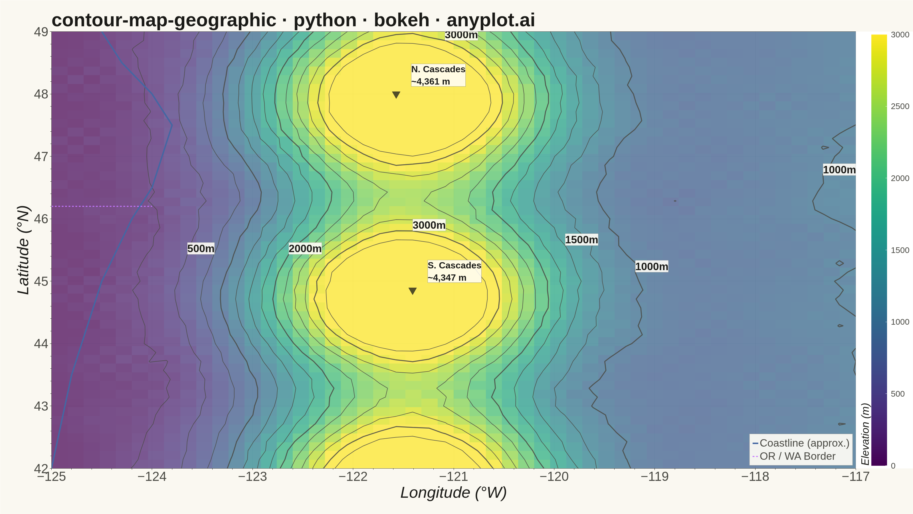
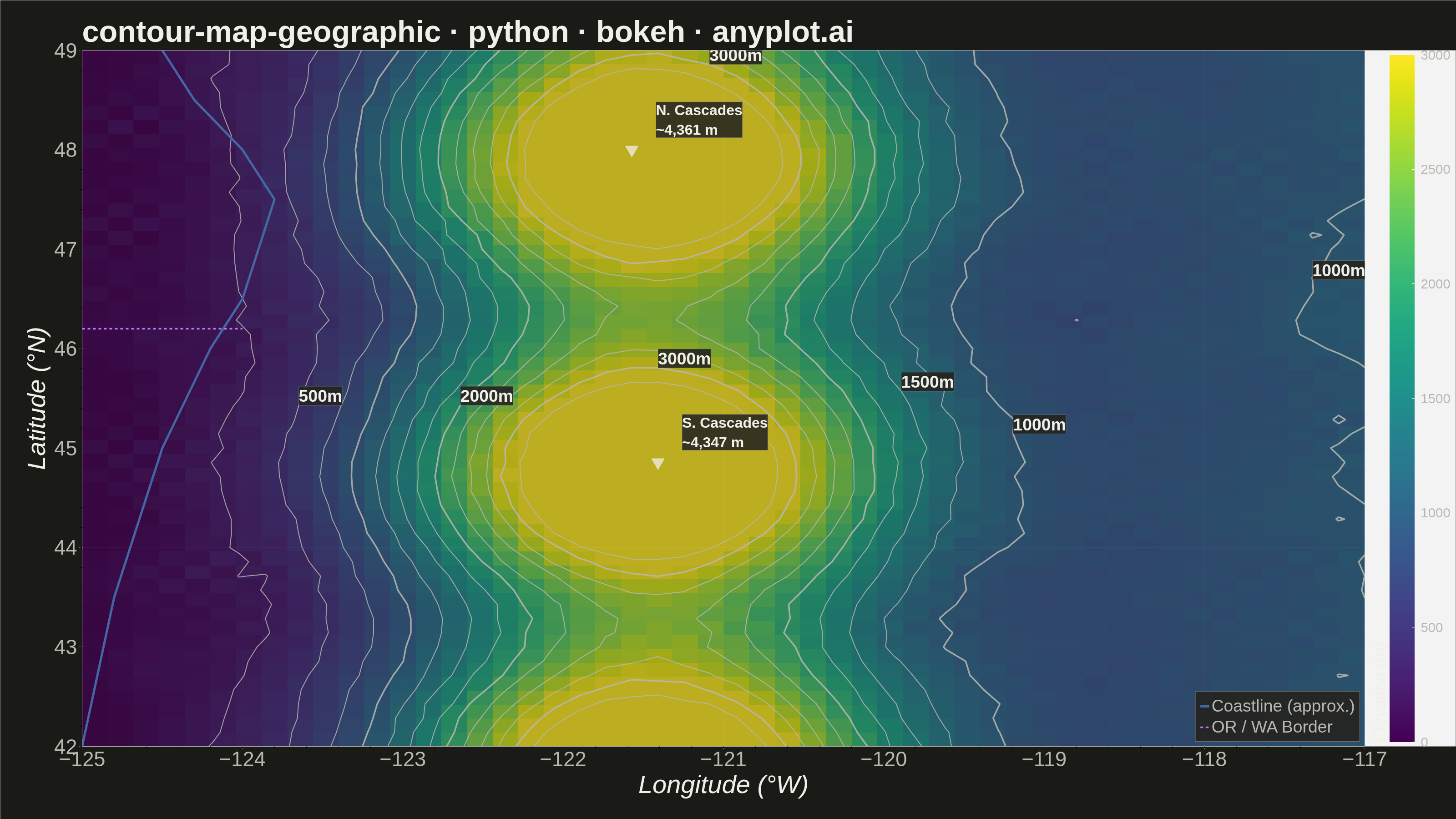
A contour map overlays isolines (lines of equal value) onto a geographic basemap, visualizing continuous spatial data such as elevation, temperature, or atmospheric pressure across real-world coordinates. Unlike basic contour plots that use abstract x/y coordinates, this plot anchors contours to latitude/longitude positions with geographic context like coastlines, borders, or terrain. It combines the precision of isoline visualization with spatial awareness, making it ideal for meteorological, topographic, and environmental applications.
""" anyplot.ai
contour-map-geographic: Contour Lines on Geographic Map
Library: bokeh 3.9.0 | Python 3.13.13
Quality: 88/100 | Updated: 2026-05-20
"""

import os
import sys
import time
from pathlib import Path


# Remove the current directory from sys.path to avoid shadowing the bokeh package
sys.path = [p for p in sys.path if p not in ("", ".", os.getcwd(), os.path.dirname(__file__))]

import numpy as np
from bokeh.io import output_file, save
from bokeh.models import ColorBar, ColumnDataSource, Label, LabelSet, LinearColorMapper
from bokeh.palettes import Viridis256
from bokeh.plotting import figure
from contourpy import contour_generator
from selenium import webdriver
from selenium.webdriver.chrome.options import Options


THEME = os.getenv("ANYPLOT_THEME", "light")

PAGE_BG = "#FAF8F1" if THEME == "light" else "#1A1A17"
ELEVATED_BG = "#FFFDF6" if THEME == "light" else "#242420"
INK = "#1A1A17" if THEME == "light" else "#F0EFE8"
INK_SOFT = "#4A4A44" if THEME == "light" else "#B8B7B0"

# --- Data: simulated elevation, Pacific Northwest (Oregon → Washington) ---
np.random.seed(42)

lat_min, lat_max = 42.0, 49.0
lon_min, lon_max = -125.0, -117.0

n_points = 50
lons = np.linspace(lon_min, lon_max, n_points)
lats = np.linspace(lat_min, lat_max, n_points)
lon_grid, lat_grid = np.meshgrid(lons, lats)

# Base: elevation rises west → east
base_elevation = (lon_grid - lon_min) / (lon_max - lon_min) * 1000

# Cascade Range — two-peak morphology from sin modulation
cascade_center_lon = -121.5
cascade_width = 1.0
cascade_height = np.exp(-((lon_grid - cascade_center_lon) ** 2) / (2 * cascade_width**2))
cascade_elevation = cascade_height * 3000 * (1 + 0.3 * np.sin(lat_grid * 2))

# Terrain noise (smoothed)
terrain_noise = np.random.randn(n_points, n_points) * 100
for _ in range(3):
    terrain_noise = (
        np.roll(terrain_noise, 1, axis=0)
        + np.roll(terrain_noise, -1, axis=0)
        + np.roll(terrain_noise, 1, axis=1)
        + np.roll(terrain_noise, -1, axis=1)
    ) / 4

elevation = np.clip(base_elevation + cascade_elevation + terrain_noise, 0, None)

# Find the two Cascade Range peaks for narrative annotation
north_elev = np.where(lat_grid > 46.5, elevation, 0)
north_idx = np.unravel_index(np.argmax(north_elev), north_elev.shape)
north_lat, north_lon = lats[north_idx[0]], lons[north_idx[1]]

south_elev = np.where(lat_grid <= 46.5, elevation, 0)
south_idx = np.unravel_index(np.argmax(south_elev), south_elev.shape)
south_lat, south_lon = lats[south_idx[0]], lons[south_idx[1]]

# Extract contour paths with contourpy (no matplotlib import needed here)
levels = list(np.arange(250, 3500, 250))
gen = contour_generator(x=lon_grid, y=lat_grid, z=elevation)

# --- Figure ---
W, H = 3200, 1800
p = figure(
    width=W,
    height=H,
    title="contour-map-geographic · python · bokeh · anyplot.ai",
    x_axis_label="Longitude (°W)",
    y_axis_label="Latitude (°N)",
    x_range=(lon_min, lon_max),
    y_range=(lat_min, lat_max),
    toolbar_location=None,
    tools="pan,wheel_zoom,reset",
    min_border_bottom=160,
    min_border_left=180,
    min_border_top=110,
    min_border_right=80,
)

# --- Typography ---
p.title.text_font_size = "50pt"
p.title.text_color = INK
p.xaxis.axis_label_text_font_size = "42pt"
p.yaxis.axis_label_text_font_size = "42pt"
p.xaxis.major_label_text_font_size = "34pt"
p.yaxis.major_label_text_font_size = "34pt"
p.xaxis.axis_label_text_color = INK
p.yaxis.axis_label_text_color = INK
p.xaxis.major_label_text_color = INK_SOFT
p.yaxis.major_label_text_color = INK_SOFT
p.xaxis.axis_line_color = INK_SOFT
p.yaxis.axis_line_color = INK_SOFT
p.xaxis.major_tick_line_color = INK_SOFT
p.yaxis.major_tick_line_color = INK_SOFT

# --- Background & chrome ---
p.background_fill_color = PAGE_BG
p.border_fill_color = PAGE_BG
p.outline_line_color = INK_SOFT

p.xgrid.grid_line_color = INK
p.ygrid.grid_line_color = INK
p.xgrid.grid_line_alpha = 0.10
p.ygrid.grid_line_alpha = 0.10

# --- Elevation raster ---
color_mapper = LinearColorMapper(palette=Viridis256, low=0, high=3000)
p.image(
    image=[elevation],
    x=lon_min,
    y=lat_min,
    dw=lon_max - lon_min,
    dh=lat_max - lat_min,
    color_mapper=color_mapper,
    alpha=0.72,
)

# --- Contour lines with overlap-aware label placement ---
MIN_LABEL_DIST = 0.8  # minimum degrees between elevation label centers
label_data = {"x": [], "y": [], "text": []}
for level in levels:
    paths = gen.lines(level)
    for path in paths:
        if path is None or len(path) < 5:
            continue
        line_width = 3.5 if level % 1000 == 0 else 2.0
        p.line(x=path[:, 0], y=path[:, 1], line_color=INK_SOFT, line_width=line_width, line_alpha=0.85)
        if level % 500 == 0 and len(path) > 20:
            mid = len(path) // 2
            cx, cy = path[mid, 0], path[mid, 1]
            too_close = any(
                (cx - ex) ** 2 + (cy - ey) ** 2 < MIN_LABEL_DIST**2
                for ex, ey in zip(label_data["x"], label_data["y"], strict=False)
            )
            if not too_close:
                label_data["x"].append(cx)
                label_data["y"].append(cy)
                label_data["text"].append(f"{int(level)}m")

# --- Contour elevation labels ---
label_source = ColumnDataSource(data=label_data)
labels = LabelSet(
    x="x",
    y="y",
    text="text",
    source=label_source,
    text_font_size="28pt",
    text_color=INK,
    text_font_style="bold",
    background_fill_color=ELEVATED_BG,
    background_fill_alpha=0.90,
    border_line_color=INK_SOFT,
    border_line_alpha=0.35,
)
p.add_layout(labels)

# --- Approximate Pacific coastline (Okabe-Ito #4467A3: blue = water, semantically justified) ---
coast_lons = [-125.0, -124.8, -124.5, -124.2, -124.0, -123.8, -124.0, -124.3, -124.5]
coast_lats = [42.0, 43.5, 45.0, 46.0, 46.5, 47.5, 48.0, 48.5, 49.0]
p.line(x=coast_lons, y=coast_lats, line_color="#4467A3", line_width=5, legend_label="Coastline (approx.)")

# --- Oregon / Washington state border (lat ≈ 46.2) for geographic context ---
p.line(
    x=[lon_min, -124.0],
    y=[46.2, 46.2],
    line_color="#C475FD",  # Okabe-Ito orange
    line_width=3.5,
    line_dash="dashed",
    legend_label="OR / WA Border",
)

# --- Cascade Range peak markers and annotations for geographic narrative ---
for peak_lon, peak_lat, peak_elev, name in [
    (south_lon, south_lat, int(elevation[south_idx]), "S. Cascades"),
    (north_lon, north_lat, int(elevation[north_idx]), "N. Cascades"),
]:
    p.add_layout(
        Label(
            x=peak_lon + 0.15,
            y=peak_lat + 0.12,
            text=f"{name}\n~{peak_elev:,} m",
            text_font_size="24pt",
            text_color=INK,
            text_font_style="bold",
            background_fill_color=ELEVATED_BG,
            background_fill_alpha=0.88,
            border_line_color=INK_SOFT,
            border_line_alpha=0.5,
        )
    )
p.scatter(
    x=[south_lon, north_lon], y=[south_lat, north_lat], marker="inverted_triangle", size=28, color=INK, alpha=0.75
)

# --- Colorbar ---
color_bar = ColorBar(
    color_mapper=color_mapper,
    label_standoff=14,
    width=55,
    location=(0, 0),
    title="Elevation (m)",
    title_text_font_size="28pt",
    title_text_color=INK,
    major_label_text_font_size="22pt",
    major_label_text_color=INK_SOFT,
)
p.add_layout(color_bar, "right")

# --- Legend ---
p.legend.location = "bottom_right"
p.legend.label_text_font_size = "28pt"
p.legend.label_text_color = INK_SOFT
p.legend.background_fill_color = ELEVATED_BG
p.legend.border_line_color = INK_SOFT
p.legend.background_fill_alpha = 0.92

# --- Save HTML + PNG via headless Chrome ---
output_file(f"plot-{THEME}.html")
save(p)

opts = Options()
for arg in (
    "--headless=new",
    "--no-sandbox",
    "--disable-dev-shm-usage",
    "--disable-gpu",
    f"--window-size={W},{H}",
    "--hide-scrollbars",
):
    opts.add_argument(arg)

driver = webdriver.Chrome(options=opts)
driver.execute_cdp_cmd(
    "Emulation.setDeviceMetricsOverride", {"width": W, "height": H, "deviceScaleFactor": 1, "mobile": False}
)
driver.get(f"file://{Path(f'plot-{THEME}.html').resolve()}")
time.sleep(3)
driver.save_screenshot(f"plot-{THEME}.png")
driver.quit()
Runnable source as JSON, for any HTTP client: https://api.anyplot.ai/specs/contour-map-geographic/bokeh/code. Any spec id and library id listed in llms-full.txt fit the same URL shape; every URL below is complete and callable.
{
  "spec_id": "contour-map-geographic",
  "language": "python",
  "library": "bokeh",
  "page": "https://anyplot.ai/contour-map-geographic/python/bokeh",
  "hub": "https://anyplot.ai/contour-map-geographic",
  "code_json": "https://api.anyplot.ai/specs/contour-map-geographic/bokeh/code",
  "spec_json": "https://api.anyplot.ai/specs/contour-map-geographic",
  "render_light_png": "https://storage.googleapis.com/anyplot-images/plots/contour-map-geographic/python/bokeh/plot-light.png",
  "render_dark_png": "https://storage.googleapis.com/anyplot-images/plots/contour-map-geographic/python/bokeh/plot-dark.png",
  "interactive_light_html": "https://storage.googleapis.com/anyplot-images/plots/contour-map-geographic/python/bokeh/plot-light.html",
  "interactive_dark_html": "https://storage.googleapis.com/anyplot-images/plots/contour-map-geographic/python/bokeh/plot-dark.html",
  "quality_score": 88.0,
  "license": "MIT",
  "guide": "https://anyplot.ai/llms.txt"
}
Part of Contour Lines on Geographic Map on anyplot.ai.