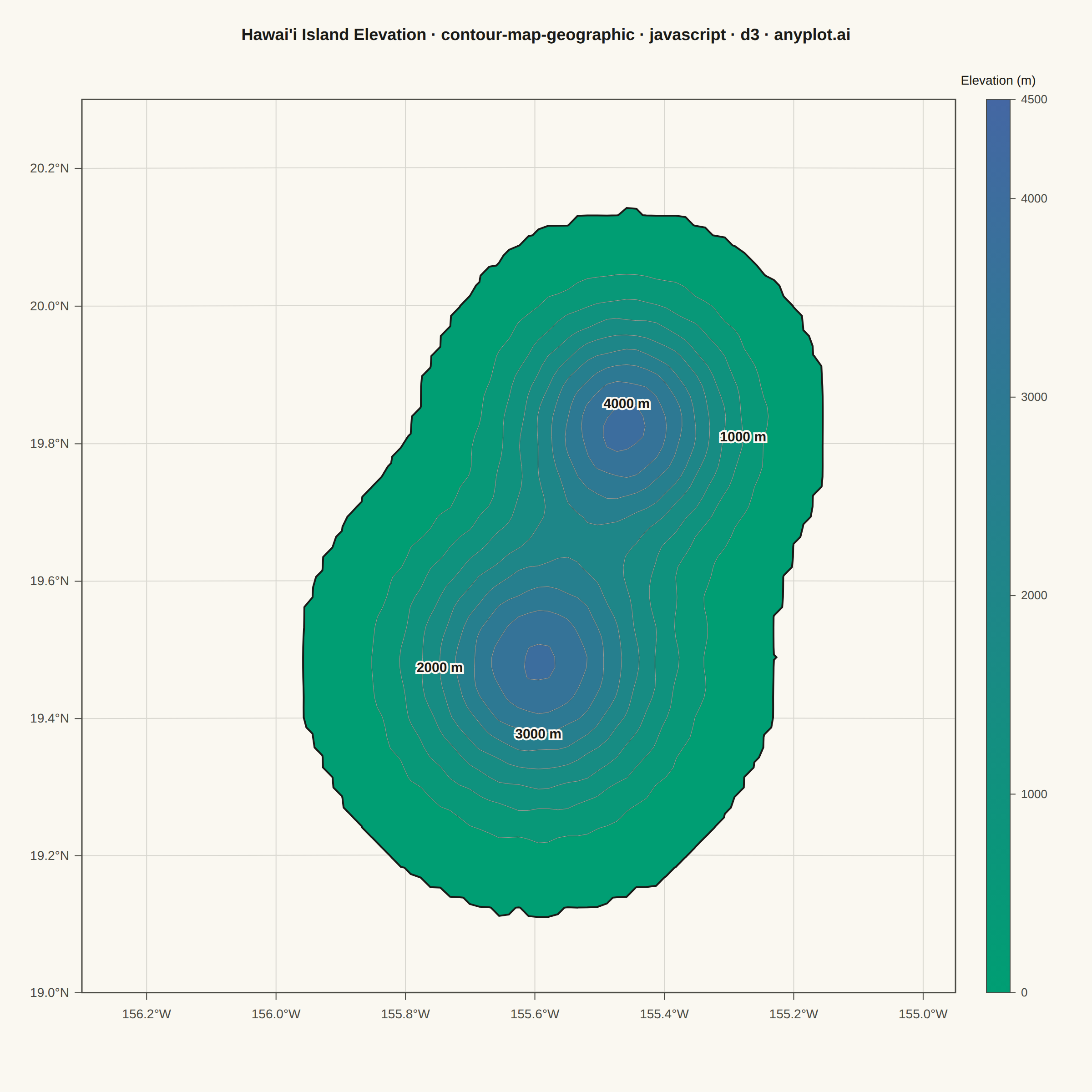
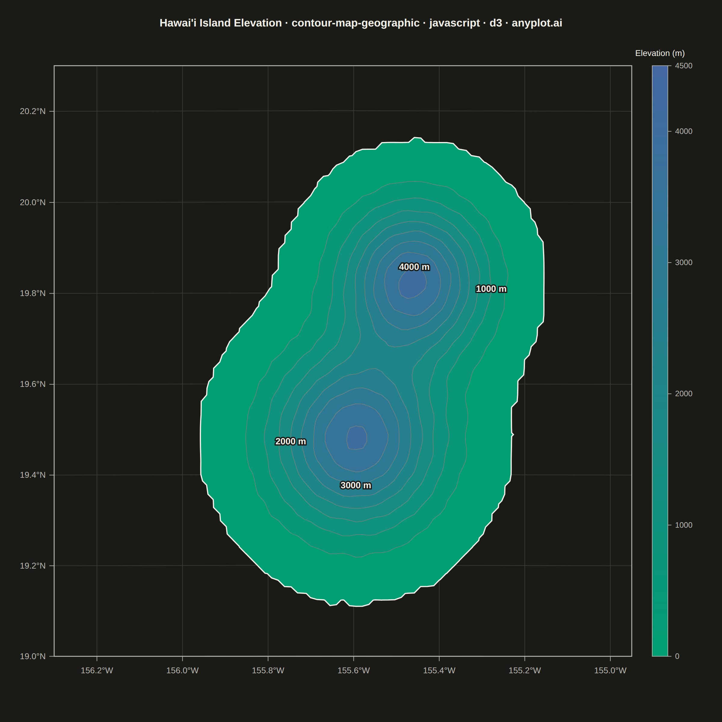
The same plot in 14 other libraries — JavaScript: Chart.js, Apache ECharts, Highcharts, MUI X Charts; Python: Altair, Bokeh, lets-plot, Matplotlib, Plotly, plotnine, Pygal, Seaborn; R: ggplot2; Julia: Makie.jl. Compare all 15 side by side: Contour Lines on Geographic Map in Python, R, Julia and JavaScript.
A contour map overlays isolines (lines of equal value) onto a geographic basemap, visualizing continuous spatial data such as elevation, temperature, or atmospheric pressure across real-world coordinates. Unlike basic contour plots that use abstract x/y coordinates, this plot anchors contours to latitude/longitude positions with geographic context like coastlines, borders, or terrain. It combines the precision of isoline visualization with spatial awareness, making it ideal for meteorological, topographic, and environmental applications.
// anyplot.ai
// contour-map-geographic: Contour Lines on Geographic Map
// Library: d3 7.9.0 | JavaScript 22.23.2
// Quality: 90/100 | Created: 2026-09-01

//# anyplot-orientation: square
const t = window.ANYPLOT_TOKENS;
const { width, height } = window.ANYPLOT_SIZE;
// Hawai'i Island's bbox is nearly square (lon range 1.35 deg x cos(19.6 deg)
// = 1.27 deg vs. lat range 1.3 deg), so a square canvas lets the map fill the
// frame instead of being stranded inside a 16:9 landscape with dead margins.
const margin = { top: 90, right: 150, bottom: 90, left: 90 };

// --- Data: synthetic elevation model of Hawai'i Island (Big Island) --------
// Two shield-volcano summits near the real Mauna Kea / Mauna Loa positions,
// plus deterministic ridge texture. A sea-level floor at base=90 carves a
// closed 0 m coastline out of the smooth terrain — no external DEM needed.
// The bounding box is padded well beyond both summits so every isoline closes
// inside the frame instead of being clipped by the domain edge.
const LON_MIN = -156.3;
const LON_MAX = -154.95;
const LAT_MIN = 19.0;
const LAT_MAX = 20.3;
const NX = 90;
const NY = 90;

const peaks = [
  { lon: -155.4681, lat: 19.8207, elevation: 4207, spread: 0.11 }, // Mauna Kea
  { lon: -155.602, lat: 19.4721, elevation: 4169, spread: 0.13 }, // Mauna Loa
];

const grid = new Float64Array(NX * NY);
for (let j = 0; j < NY; j++) {
  const lat = LAT_MIN + (j / (NY - 1)) * (LAT_MAX - LAT_MIN);
  for (let i = 0; i < NX; i++) {
    const lon = LON_MIN + (i / (NX - 1)) * (LON_MAX - LON_MIN);
    let base = 0;
    for (const p of peaks) {
      const d2 = (lon - p.lon) ** 2 + (lat - p.lat) ** 2;
      base += p.elevation * Math.exp(-d2 / (2 * p.spread * p.spread));
    }
    // Ridge texture fades to zero away from the summits, so it can't push
    // isolated low-lying ocean cells above the coastline threshold.
    const ridgeMask = Math.min(1, base / 600);
    const ridgeTexture = 45 * Math.sin(lon * 90) * Math.cos(lat * 70) * ridgeMask;
    grid[j * NX + i] = Math.max(0, base + ridgeTexture - 90); // sea-level cutoff
  }
}
const maxElevation = d3.max(grid);

// --- Contours (grid-index space -> lon/lat) ---------------------------------
const STEP = 500;
const maxBand = Math.ceil(maxElevation / STEP) * STEP;
const thresholds = [1];
for (let v = STEP; v <= maxBand; v += STEP) thresholds.push(v);

const contoursGeo = d3
  .contours()
  .size([NX, NY])
  .thresholds(thresholds)(grid)
  .map((c) => ({
    type: "MultiPolygon",
    value: c.value,
    coordinates: c.coordinates.map((poly) =>
      poly.map((ring) =>
        ring.map(([x, y]) => [
          LON_MIN + (x / (NX - 1)) * (LON_MAX - LON_MIN),
          LAT_MIN + (y / (NY - 1)) * (LAT_MAX - LAT_MIN),
        ]),
      ),
    ),
  }));

// --- Projection fitted to the region, inside the margin box -----------------
// Ring wound so d3-geo's spherical right-hand rule reads this as the small
// interior bbox (not its complement covering the rest of the globe).
const bboxFeature = {
  type: "Polygon",
  coordinates: [
    [
      [LON_MIN, LAT_MIN],
      [LON_MIN, LAT_MAX],
      [LON_MAX, LAT_MAX],
      [LON_MAX, LAT_MIN],
      [LON_MIN, LAT_MIN],
    ],
  ],
};
const projection = d3
  .geoMercator()
  .fitExtent(
    [
      [margin.left, margin.top],
      [width - margin.right, height - margin.bottom],
    ],
    bboxFeature,
  );
const geoPath = d3.geoPath(projection);

const corners = bboxFeature.coordinates[0].map(projection);
const mapX0 = d3.min(corners, (d) => d[0]);
const mapX1 = d3.max(corners, (d) => d[0]);
const mapY0 = d3.min(corners, (d) => d[1]);
const mapY1 = d3.max(corners, (d) => d[1]);

// --- Color: single-polarity elevation -> imprint_seq -------------------------
const colorScale = d3.scaleSequential(d3.interpolateRgbBasis(t.seq)).domain([0, maxBand]);

// --- SVG mount ----------------------------------------------------------------
const svg = d3.select("#container").append("svg").attr("width", width).attr("height", height);

// Lon/lat graticule (drawn first, visible over the ocean background)
const graticule = d3.geoGraticule().extent([
  [LON_MIN, LAT_MIN],
  [LON_MAX, LAT_MAX],
]).step([0.2, 0.2]);
svg
  .append("path")
  .datum(graticule())
  .attr("d", geoPath)
  .attr("fill", "none")
  .attr("stroke", t.grid)
  .attr("stroke-width", 1);

// Filled elevation bands, painted ascending so each nested level overwrites
// the wider band beneath it — turns the "value >= threshold" isoband stack
// from d3-contour into a proper stepped hypsometric fill.
const bandGroup = svg.append("g");
for (const c of contoursGeo) {
  bandGroup
    .append("path")
    .datum(c)
    .attr("d", geoPath)
    .attr("fill", colorScale(c.value))
    .attr("stroke", t.pageBg)
    .attr("stroke-width", 0.5);
}

// Isoline strokes on top of the fills (line-only contour detail)
for (const c of contoursGeo.slice(1)) {
  svg
    .append("path")
    .datum(c)
    .attr("d", geoPath)
    .attr("fill", "none")
    .attr("stroke", t.inkSoft)
    .attr("stroke-width", 1)
    .attr("stroke-opacity", 0.5);
}

// Coastline (0 m isoline) emphasized as the map's geographic anchor
svg
  .append("path")
  .datum(contoursGeo[0])
  .attr("d", geoPath)
  .attr("fill", "none")
  .attr("stroke", t.ink)
  .attr("stroke-width", 2);

// Contour value labels at meaningful elevation intervals. Some bands merge
// into one ring around both summits, others split into two disjoint rings —
// so each label reads off the ring's extreme point in a distinct compass
// direction (E/W/S/N) rather than an arc fraction, which keeps callouts
// spread around the island's open flanks instead of stacking near a peak.
const LABEL_VALUES = [1000, 2000, 3000, 4000];
const LABEL_DIRECTIONS = [
  [0, 1], // 1000 m -> easternmost point (max lon)
  [0, -1], // 2000 m -> westernmost point (min lon)
  [1, -1], // 3000 m -> southernmost point (min lat)
  [1, 1], // 4000 m -> northernmost point (max lat)
];
LABEL_VALUES.forEach((val, i) => {
  const c = contoursGeo.find((d) => d.value === val);
  if (!c) return;
  const [axis, dir] = LABEL_DIRECTIONS[i];
  let best = null;
  for (const poly of c.coordinates) {
    for (const ring of poly) {
      for (const pt of ring) {
        if (!best || pt[axis] * dir > best[axis] * dir) best = pt;
      }
    }
  }
  const [lon, lat] = best;
  const [px, py] = projection([lon, lat]);
  svg
    .append("text")
    .attr("x", px)
    .attr("y", py)
    .attr("text-anchor", "middle")
    .attr("dy", "0.35em")
    .style("font-size", "15px")
    .style("font-weight", "600")
    .style("paint-order", "stroke")
    .style("stroke", t.pageBg)
    .style("stroke-width", "4px")
    .attr("fill", t.ink)
    .text(`${val} m`);
});

// Map frame
svg
  .append("rect")
  .attr("x", mapX0)
  .attr("y", mapY0)
  .attr("width", mapX1 - mapX0)
  .attr("height", mapY1 - mapY0)
  .attr("fill", "none")
  .attr("stroke", t.inkSoft)
  .attr("stroke-width", 1.5);

// Longitude ticks (bottom) and latitude ticks (left)
const lonTicks = d3.range(Math.ceil(LON_MIN / 0.2) * 0.2, LON_MAX, 0.2);
const latTicks = d3.range(Math.ceil(LAT_MIN / 0.2) * 0.2, LAT_MAX, 0.2);

for (const lon of lonTicks) {
  const [px] = projection([lon, LAT_MIN]);
  svg
    .append("line")
    .attr("x1", px)
    .attr("x2", px)
    .attr("y1", mapY1)
    .attr("y2", mapY1 + 8)
    .attr("stroke", t.inkSoft)
    .attr("stroke-width", 1);
  svg
    .append("text")
    .attr("x", px)
    .attr("y", mapY1 + 28)
    .attr("text-anchor", "middle")
    .style("font-size", "14px")
    .attr("fill", t.inkSoft)
    .text(`${Math.abs(lon).toFixed(1)}°W`);
}

for (const lat of latTicks) {
  const [, py] = projection([LON_MIN, lat]);
  svg
    .append("line")
    .attr("x1", mapX0 - 8)
    .attr("x2", mapX0)
    .attr("y1", py)
    .attr("y2", py)
    .attr("stroke", t.inkSoft)
    .attr("stroke-width", 1);
  svg
    .append("text")
    .attr("x", mapX0 - 14)
    .attr("y", py)
    .attr("text-anchor", "end")
    .attr("dy", "0.32em")
    .style("font-size", "14px")
    .attr("fill", t.inkSoft)
    .text(`${lat.toFixed(1)}°N`);
}

// Colorbar legend — hugs the map's actual right edge instead of the margin
// box, so there's no dead gap on near-square geographic bboxes.
const barWidth = 26;
const barX = mapX1 + 34;
const barY0 = mapY0;
const barY1 = mapY1;

const gradientId = "elevationGradient";
const defs = svg.append("defs");
const gradient = defs
  .append("linearGradient")
  .attr("id", gradientId)
  .attr("x1", "0%")
  .attr("y1", "100%")
  .attr("x2", "0%")
  .attr("y2", "0%");
const stopCount = 6;
for (let i = 0; i <= stopCount; i++) {
  const f = i / stopCount;
  gradient
    .append("stop")
    .attr("offset", `${f * 100}%`)
    .attr("stop-color", colorScale(f * maxBand));
}

svg
  .append("text")
  .attr("x", barX + barWidth / 2)
  .attr("y", barY0 - 16)
  .attr("text-anchor", "middle")
  .style("font-size", "14px")
  .attr("fill", t.ink)
  .text("Elevation (m)");

svg
  .append("rect")
  .attr("x", barX)
  .attr("y", barY0)
  .attr("width", barWidth)
  .attr("height", barY1 - barY0)
  .attr("fill", `url(#${gradientId})`)
  .attr("stroke", t.inkSoft)
  .attr("stroke-width", 1);

// Includes maxBand itself so the top of the gradient always carries a label,
// even when it falls between the round 1000 m steps (e.g. 4500).
const colorbarTicks = d3.range(0, maxBand, 1000).concat(maxBand);
for (const val of colorbarTicks) {
  const y = barY1 - (val / maxBand) * (barY1 - barY0);
  svg
    .append("line")
    .attr("x1", barX + barWidth)
    .attr("x2", barX + barWidth + 6)
    .attr("y1", y)
    .attr("y2", y)
    .attr("stroke", t.inkSoft)
    .attr("stroke-width", 1);
  svg
    .append("text")
    .attr("x", barX + barWidth + 12)
    .attr("y", y)
    .attr("dy", "0.32em")
    .style("font-size", "13px")
    .attr("fill", t.inkSoft)
    .text(val);
}

// Title — scaled down from the 67-char baseline for this longer title
const titleText =
  "Hawai'i Island Elevation · contour-map-geographic · javascript · d3 · anyplot.ai";
const titleRatio = titleText.length > 67 ? 67 / titleText.length : 1;
const titleFontSize = Math.max(14, Math.round(22 * titleRatio));
svg
  .append("text")
  .attr("x", width / 2)
  .attr("y", 44)
  .attr("text-anchor", "middle")
  .attr("fill", t.ink)
  .style("font-size", `${titleFontSize}px`)
  .style("font-weight", "600")
  .text(titleText);
Runnable source as JSON, for any HTTP client: https://api.anyplot.ai/specs/contour-map-geographic/d3/code. Any spec id and library id listed in llms-full.txt fit the same URL shape; every URL below is complete and callable.
{
  "spec_id": "contour-map-geographic",
  "language": "javascript",
  "library": "d3",
  "page": "https://anyplot.ai/contour-map-geographic/javascript/d3",
  "hub": "https://anyplot.ai/contour-map-geographic",
  "code_json": "https://api.anyplot.ai/specs/contour-map-geographic/d3/code",
  "spec_json": "https://api.anyplot.ai/specs/contour-map-geographic",
  "render_light_png": "https://storage.googleapis.com/anyplot-images/plots/contour-map-geographic/javascript/d3/plot-light.png",
  "render_dark_png": "https://storage.googleapis.com/anyplot-images/plots/contour-map-geographic/javascript/d3/plot-dark.png",
  "interactive_light_html": "https://storage.googleapis.com/anyplot-images/plots/contour-map-geographic/javascript/d3/plot-light.html",
  "interactive_dark_html": "https://storage.googleapis.com/anyplot-images/plots/contour-map-geographic/javascript/d3/plot-dark.html",
  "quality_score": 90.0,
  "license": "MIT",
  "guide": "https://anyplot.ai/llms.txt"
}
Part of Contour Lines on Geographic Map on anyplot.ai.