The same plot in 14 other libraries — Python: Altair, Bokeh, lets-plot, Matplotlib, Plotly, plotnine, Pygal, Seaborn; R: ggplot2; JavaScript: Chart.js, D3.js, Apache ECharts, Highcharts, MUI X Charts. Compare all 15 side by side: Density Plot with Rug Marks in Python, R, Julia and JavaScript.
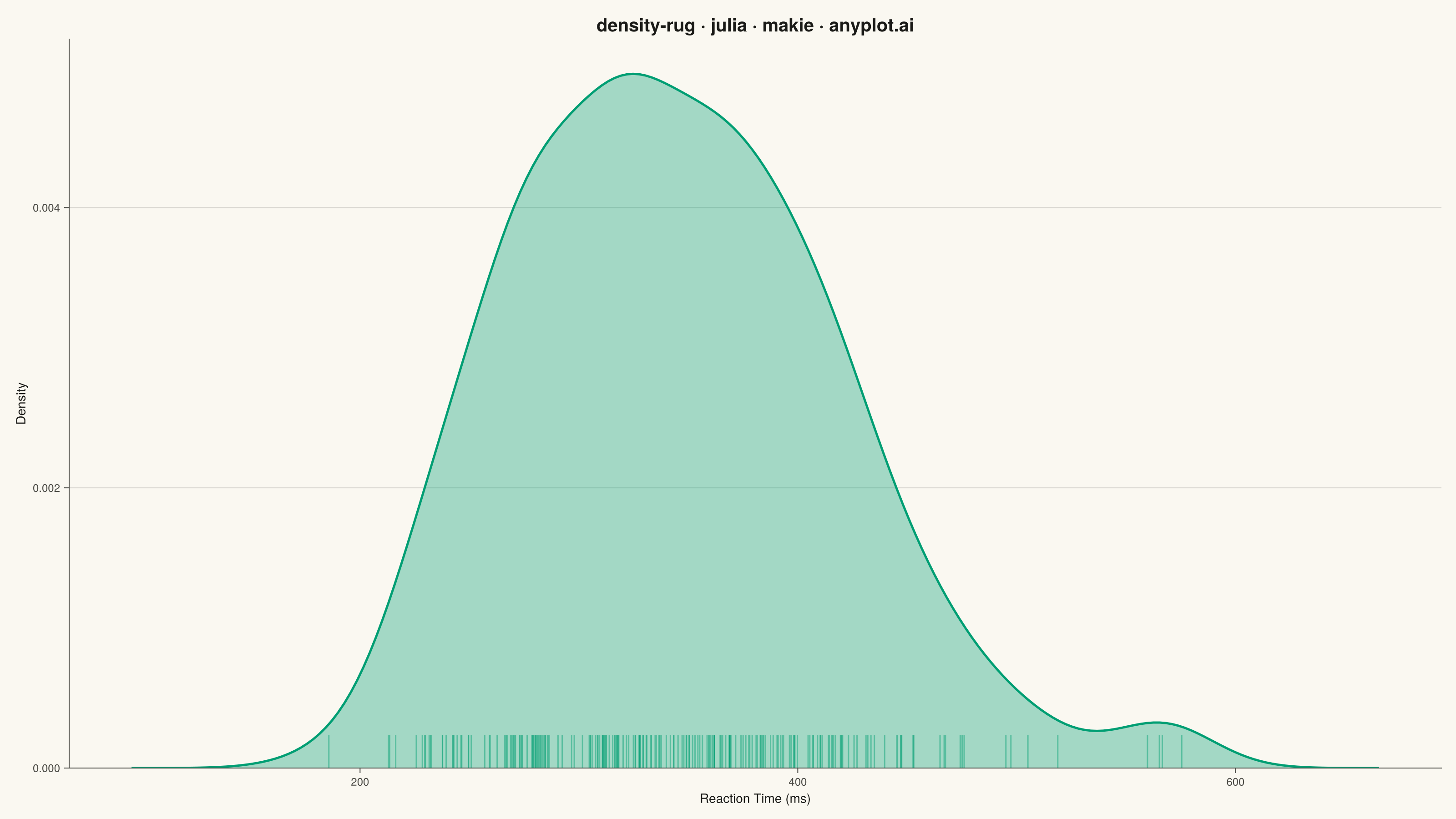
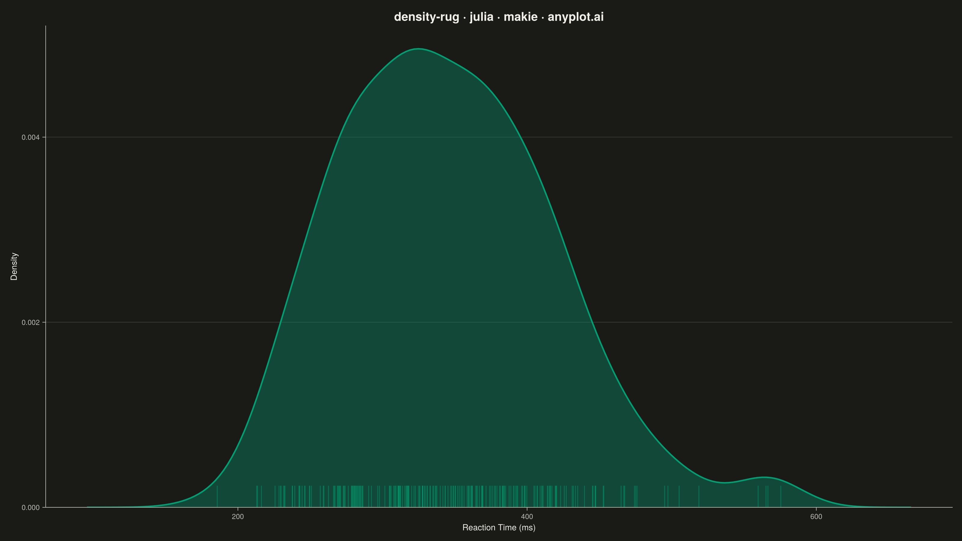
A kernel density estimation (KDE) plot combined with rug marks along the x-axis, showing both the smoothed probability distribution and the exact location of each individual data point. This combination provides the best of both worlds: the KDE reveals the overall shape, modality, and smoothed density of the distribution, while the rug marks preserve transparency about where actual observations fall, highlighting data density and potential gaps.
# anyplot.ai
# density-rug: Density Plot with Rug Marks
# Library: makie 0.21.9 | Julia 1.11.9
# Quality: 82/100 | Created: 2026-09-02

using CairoMakie
using Colors
using Random
using Statistics

Random.seed!(42)

# --- Theme tokens -----------------------------------------------------------
THEME    = get(ENV, "ANYPLOT_THEME", "light")
PAGE_BG  = THEME == "light" ? colorant"#FAF8F1" : colorant"#1A1A17"
INK      = THEME == "light" ? colorant"#1A1A17" : colorant"#F0EFE8"
INK_SOFT = THEME == "light" ? colorant"#4A4A44" : colorant"#B8B7B0"
BRAND    = colorant"#009E73"  # Imprint palette position 1 — always first series

# --- Data ---------------------------------------------------------------
# Reaction times (ms) from a cognitive test battery: a large cluster of
# typical trials plus a smaller cluster of attentional lapses (slow-response
# outliers), giving the KDE a genuine second mode for the rug to corroborate.
n_typical = 190
n_lapses  = 30
typical_times_ms = exp.(0.18 .* randn(n_typical) .+ log(330))
lapse_times_ms   = exp.(0.10 .* randn(n_lapses) .+ log(580))
reaction_times_ms = vcat(typical_times_ms, lapse_times_ms)

# Valley between the two modes — used to graduate emphasis toward the tail.
mode_split = (median(typical_times_ms) + median(lapse_times_ms)) / 2

# Manual Gaussian KDE (Silverman bandwidth) so the fill/stroke can be split
# into a layered `band!` composition instead of one flat `density!` shape.
function silverman_bandwidth(x)
    n = length(x)
    iqr = quantile(x, 0.75) - quantile(x, 0.25)
    return 0.9 * min(std(x), iqr / 1.34) * n^(-1 / 5)
end

function gaussian_kde(x, grid, bandwidth)
    y = zeros(length(grid))
    for xi in x
        @. y += exp(-0.5 * ((grid - xi) / bandwidth)^2)
    end
    return y ./ (length(x) * bandwidth * sqrt(2π))
end

bandwidth = silverman_bandwidth(reaction_times_ms)
grid_lo   = max(0.0, minimum(reaction_times_ms) - 3bandwidth)
grid_hi   = maximum(reaction_times_ms) + 3bandwidth
grid      = collect(range(grid_lo, grid_hi; length = 400))
density_y = gaussian_kde(reaction_times_ms, grid, bandwidth)

typical_mask = grid .<= mode_split
lapse_mask   = grid .>= mode_split

# --- Plot ---------------------------------------------------------------
fig = Figure(
    resolution      = (1600, 900),
    fontsize        = 14,
    backgroundcolor = PAGE_BG,
)

ax = Axis(
    fig[1, 1];
    title              = "density-rug · julia · makie · anyplot.ai",
    titlesize          = 23,
    titlecolor         = INK,
    xlabel             = "Reaction Time (ms)",
    ylabel             = "Density",
    xlabelsize         = 14,
    ylabelsize         = 14,
    xlabelcolor        = INK,
    ylabelcolor        = INK,
    xticklabelsize     = 12,
    yticklabelsize     = 12,
    xticklabelcolor    = INK_SOFT,
    yticklabelcolor    = INK_SOFT,
    xtickcolor         = INK_SOFT,
    ytickcolor         = INK_SOFT,
    backgroundcolor    = PAGE_BG,
    topspinevisible    = false,
    rightspinevisible  = false,
    leftspinecolor     = INK_SOFT,
    bottomspinecolor   = INK_SOFT,
    xgridvisible       = false,
    ygridcolor         = RGBAf(INK.r, INK.g, INK.b, 0.15),
    yminorgridvisible  = false,
)

# Smoothed KDE fill, layered as two `band!` passes with graduated opacity —
# lighter under the typical-trial mode, richer under the slow-response tail —
# so the secondary mode reads as a deliberate focal point rather than raw
# unemphasized shape. A single continuous stroke keeps the curve seamless,
# with a bolder overlay reinforcing the emphasis over the tail.
band!(ax, grid[typical_mask], 0, density_y[typical_mask]; color = (BRAND, 0.22))
band!(ax, grid[lapse_mask], 0, density_y[lapse_mask]; color = (BRAND, 0.55))
lines!(ax, grid, density_y; color = BRAND, linewidth = 2.5)
lines!(ax, grid[lapse_mask], density_y[lapse_mask]; color = BRAND, linewidth = 3.5)

# Rug marks — one tick per raw observation, drawn along the axis baseline in
# axis-relative units so they sit clear of the density fill. Thin, faint
# ticks keep the crowded typical-trial band legible; bolder, more opaque
# ticks over the sparse lapse tail echo the fill's emphasis.
vlines!(
    ax, typical_times_ms;
    ymin      = 0.0,
    ymax      = 0.045,
    color     = (BRAND, 0.28),
    linewidth = 1.1,
)
vlines!(
    ax, lapse_times_ms;
    ymin      = 0.0,
    ymax      = 0.045,
    color     = (BRAND, 0.7),
    linewidth = 1.8,
)

ylims!(ax, low = 0)

# --- Save -----------------------------------------------------------------
save("plot-$(THEME).png", fig; px_per_unit = 2)
Runnable source as JSON, for any HTTP client: https://api.anyplot.ai/specs/density-rug/makie/code. Any spec id and library id listed in llms-full.txt fit the same URL shape; every URL below is complete and callable.
{
  "spec_id": "density-rug",
  "language": "julia",
  "library": "makie",
  "page": "https://anyplot.ai/density-rug/julia/makie",
  "hub": "https://anyplot.ai/density-rug",
  "code_json": "https://api.anyplot.ai/specs/density-rug/makie/code",
  "spec_json": "https://api.anyplot.ai/specs/density-rug",
  "render_light_png": "https://storage.googleapis.com/anyplot-images/plots/density-rug/julia/makie/plot-light.png",
  "render_dark_png": "https://storage.googleapis.com/anyplot-images/plots/density-rug/julia/makie/plot-dark.png",
  "quality_score": 82.0,
  "license": "MIT",
  "guide": "https://anyplot.ai/llms.txt"
}
Part of Density Plot with Rug Marks on anyplot.ai.