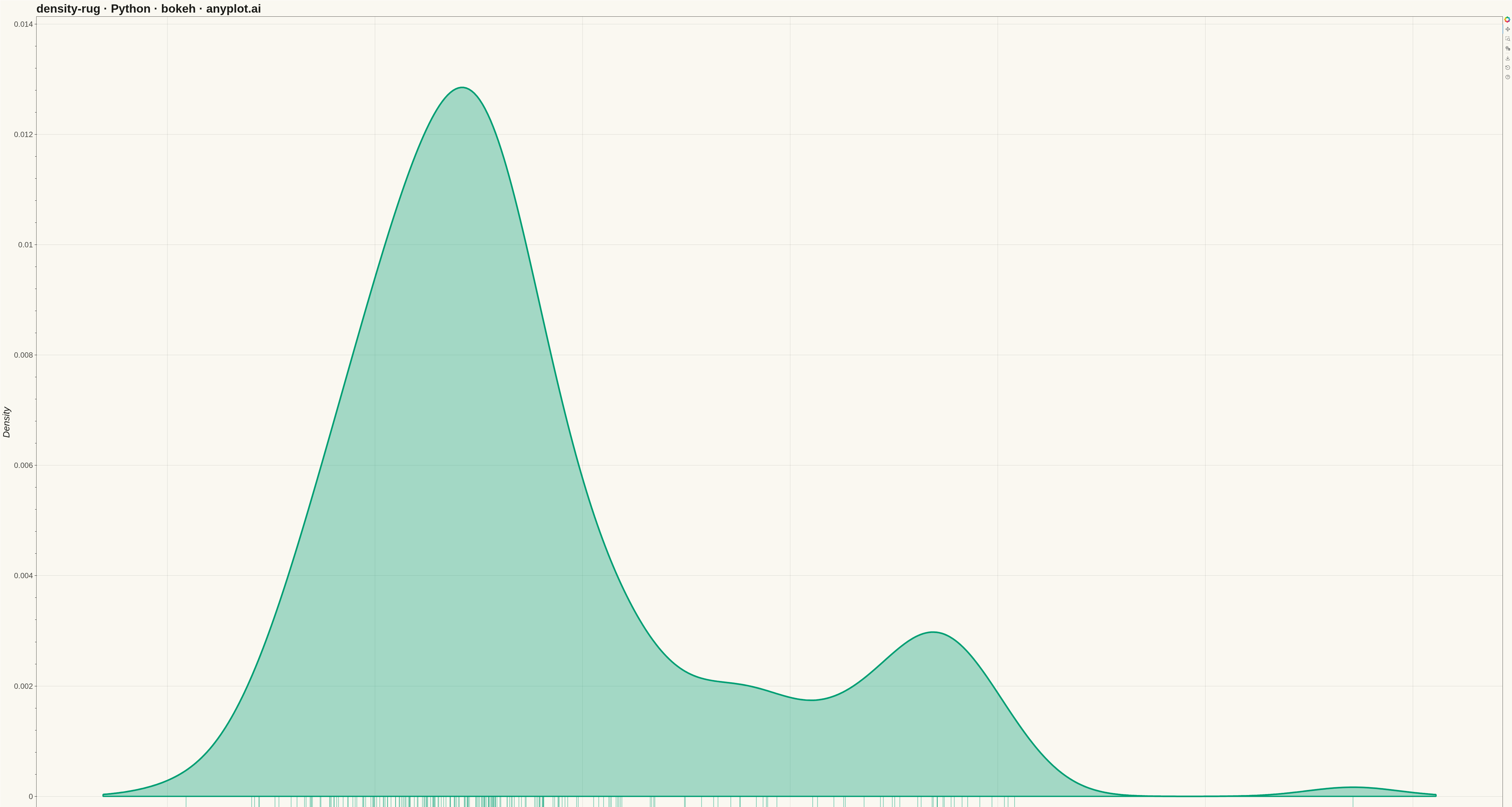
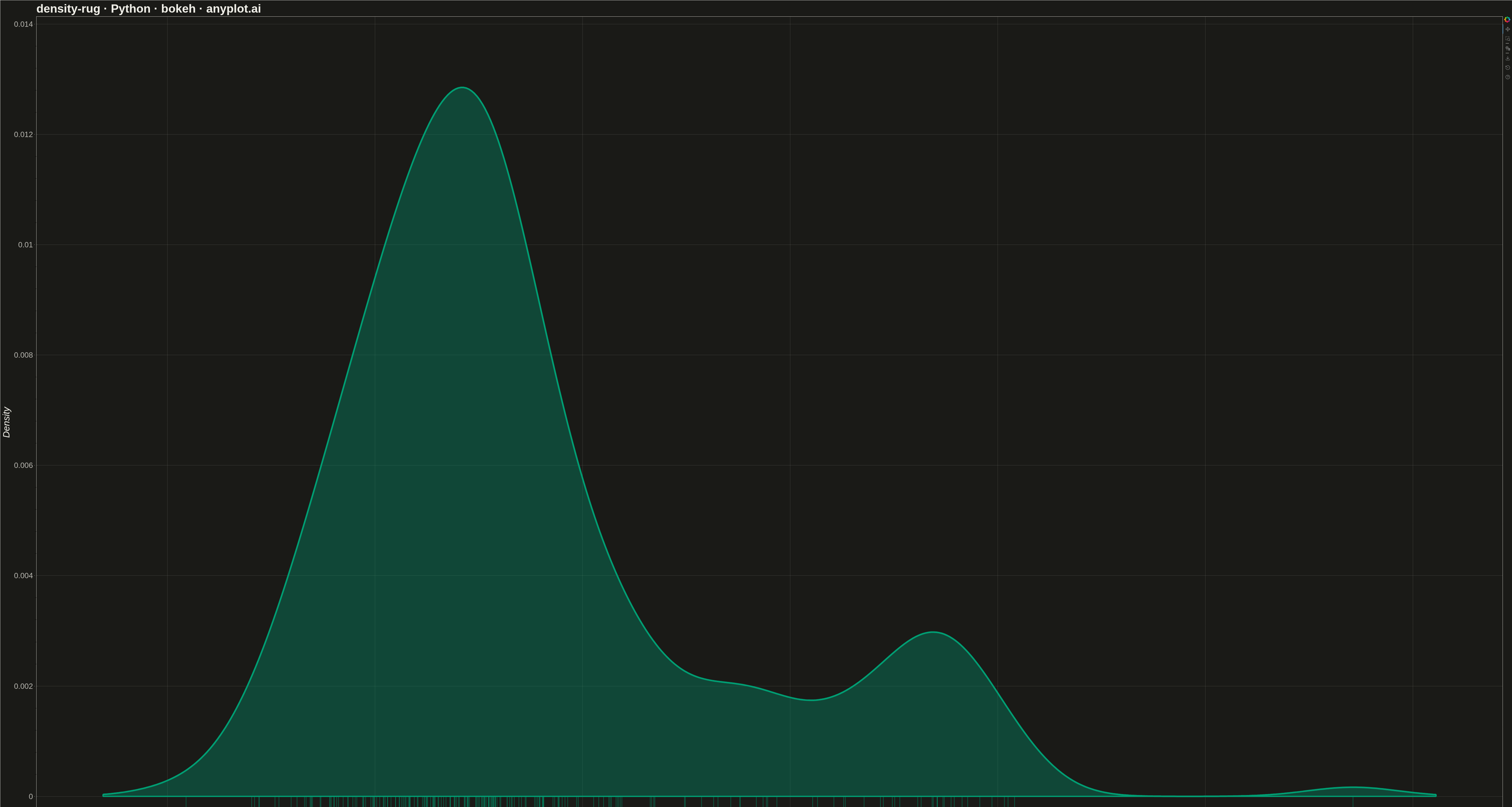
A kernel density estimation (KDE) plot combined with rug marks along the x-axis, showing both the smoothed probability distribution and the exact location of each individual data point. This combination provides the best of both worlds: the KDE reveals the overall shape, modality, and smoothed density of the distribution, while the rug marks preserve transparency about where actual observations fall, highlighting data density and potential gaps.
""" anyplot.ai
density-rug: Density Plot with Rug Marks
Library: bokeh 3.9.0 | Python 3.13.13
Quality: 95/100 | Updated: 2026-05-18
"""

import os
import time
from pathlib import Path

import numpy as np
from bokeh.models import ColumnDataSource
from bokeh.plotting import figure, output_file, save
from selenium import webdriver
from selenium.webdriver.chrome.options import Options


# Theme tokens (see prompts/default-style-guide.md)
THEME = os.getenv("ANYPLOT_THEME", "light")
PAGE_BG = "#FAF8F1" if THEME == "light" else "#1A1A17"
ELEVATED_BG = "#FFFDF6" if THEME == "light" else "#242420"
INK = "#1A1A17" if THEME == "light" else "#F0EFE8"
INK_SOFT = "#4A4A44" if THEME == "light" else "#B8B7B0"
BRAND = "#009E73"  # Okabe-Ito position 1 — ALWAYS first series

# Data - Response times in milliseconds (realistic API latency data)
np.random.seed(42)
# Mix of normal operations and some slower responses (bimodal-ish)
normal_times = np.random.normal(loc=120, scale=25, size=180)
slow_times = np.random.normal(loc=220, scale=30, size=40)
response_times = np.concatenate([normal_times, slow_times])
response_times = response_times[response_times > 0]  # Ensure positive values

# Compute KDE (Gaussian kernel density estimation)
n = len(response_times)
std = np.std(response_times)
iqr = np.percentile(response_times, 75) - np.percentile(response_times, 25)
bandwidth = 0.9 * min(std, iqr / 1.34) * n ** (-0.2)  # Silverman's rule

x_range = np.linspace(response_times.min() - 20, response_times.max() + 20, 500)
density = np.zeros_like(x_range)
for xi in response_times:
    density += np.exp(-0.5 * ((x_range - xi) / bandwidth) ** 2)
density = density / (n * bandwidth * np.sqrt(2 * np.pi))

# Create figure
p = figure(
    width=4800,
    height=2700,
    title="density-rug · Python · bokeh · anyplot.ai",
    x_axis_label="Response Time (ms)",
    y_axis_label="Density",
)

# Plot KDE as filled area using patch
kde_x = np.concatenate([[x_range[0]], x_range, [x_range[-1]]])
kde_y = np.concatenate([[0], density, [0]])
p.patch(x=kde_x, y=kde_y, fill_color=BRAND, fill_alpha=0.35, line_color=BRAND, line_width=4)

# Plot KDE line on top
kde_source = ColumnDataSource(data={"x": x_range, "y": density})
p.line(x="x", y="y", source=kde_source, line_color=BRAND, line_width=5)

# Rug marks along x-axis
rug_height = density.max() * 0.03  # Small tick height relative to density
rug_source = ColumnDataSource(
    data={"x": response_times, "y0": np.zeros(len(response_times)), "y1": np.full(len(response_times), -rug_height)}
)
p.segment(x0="x", y0="y0", x1="x", y1="y1", source=rug_source, line_color=BRAND, line_width=2, line_alpha=0.5)

# Styling - sizes for 4800x2700 canvas
p.title.text_font_size = "28pt"
p.title.text_color = INK
p.xaxis.axis_label_text_font_size = "22pt"
p.yaxis.axis_label_text_font_size = "22pt"
p.xaxis.axis_label_text_color = INK
p.yaxis.axis_label_text_color = INK
p.xaxis.major_label_text_font_size = "18pt"
p.yaxis.major_label_text_font_size = "18pt"
p.xaxis.major_label_text_color = INK_SOFT
p.yaxis.major_label_text_color = INK_SOFT

# Grid - subtle, not prominent
p.xgrid.grid_line_alpha = 0.15
p.ygrid.grid_line_alpha = 0.15
p.xgrid.grid_line_color = INK
p.ygrid.grid_line_color = INK

# Theme-adaptive chrome
p.background_fill_color = PAGE_BG
p.border_fill_color = PAGE_BG
p.outline_line_color = INK_SOFT
p.xaxis.axis_line_color = INK_SOFT
p.yaxis.axis_line_color = INK_SOFT
p.xaxis.major_tick_line_color = INK_SOFT
p.yaxis.major_tick_line_color = INK_SOFT

# Extend y-axis slightly below 0 to show rug marks
p.y_range.start = -rug_height * 1.5
p.y_range.end = density.max() * 1.1

# Save HTML
output_file(f"plot-{THEME}.html")
save(p)

# Screenshot it with headless Chrome — Selenium 4 / Selenium Manager
W, H = 4800, 2700
opts = Options()
for arg in (
    "--headless=new",
    "--no-sandbox",
    "--disable-dev-shm-usage",
    "--disable-gpu",
    f"--window-size={W},{H}",
    "--hide-scrollbars",
):
    opts.add_argument(arg)
driver = webdriver.Chrome(options=opts)
driver.set_window_size(W, H)
driver.get(f"file://{Path(f'plot-{THEME}.html').resolve()}")
time.sleep(3)  # let bokeh's JS render the canvas
driver.save_screenshot(f"plot-{THEME}.png")
driver.quit()
Runnable source as JSON, for any HTTP client: https://api.anyplot.ai/specs/density-rug/bokeh/code. Any spec id and library id listed in llms-full.txt fit the same URL shape; every URL below is complete and callable.
{
  "spec_id": "density-rug",
  "language": "python",
  "library": "bokeh",
  "page": "https://anyplot.ai/density-rug/python/bokeh",
  "hub": "https://anyplot.ai/density-rug",
  "code_json": "https://api.anyplot.ai/specs/density-rug/bokeh/code",
  "spec_json": "https://api.anyplot.ai/specs/density-rug",
  "render_light_png": "https://storage.googleapis.com/anyplot-images/plots/density-rug/python/bokeh/plot-light.png",
  "render_dark_png": "https://storage.googleapis.com/anyplot-images/plots/density-rug/python/bokeh/plot-dark.png",
  "interactive_light_html": "https://storage.googleapis.com/anyplot-images/plots/density-rug/python/bokeh/plot-light.html",
  "interactive_dark_html": "https://storage.googleapis.com/anyplot-images/plots/density-rug/python/bokeh/plot-dark.html",
  "quality_score": 95.0,
  "license": "MIT",
  "guide": "https://anyplot.ai/llms.txt"
}
Part of Density Plot with Rug Marks on anyplot.ai.