Density Plot with Rug Marks — Altair

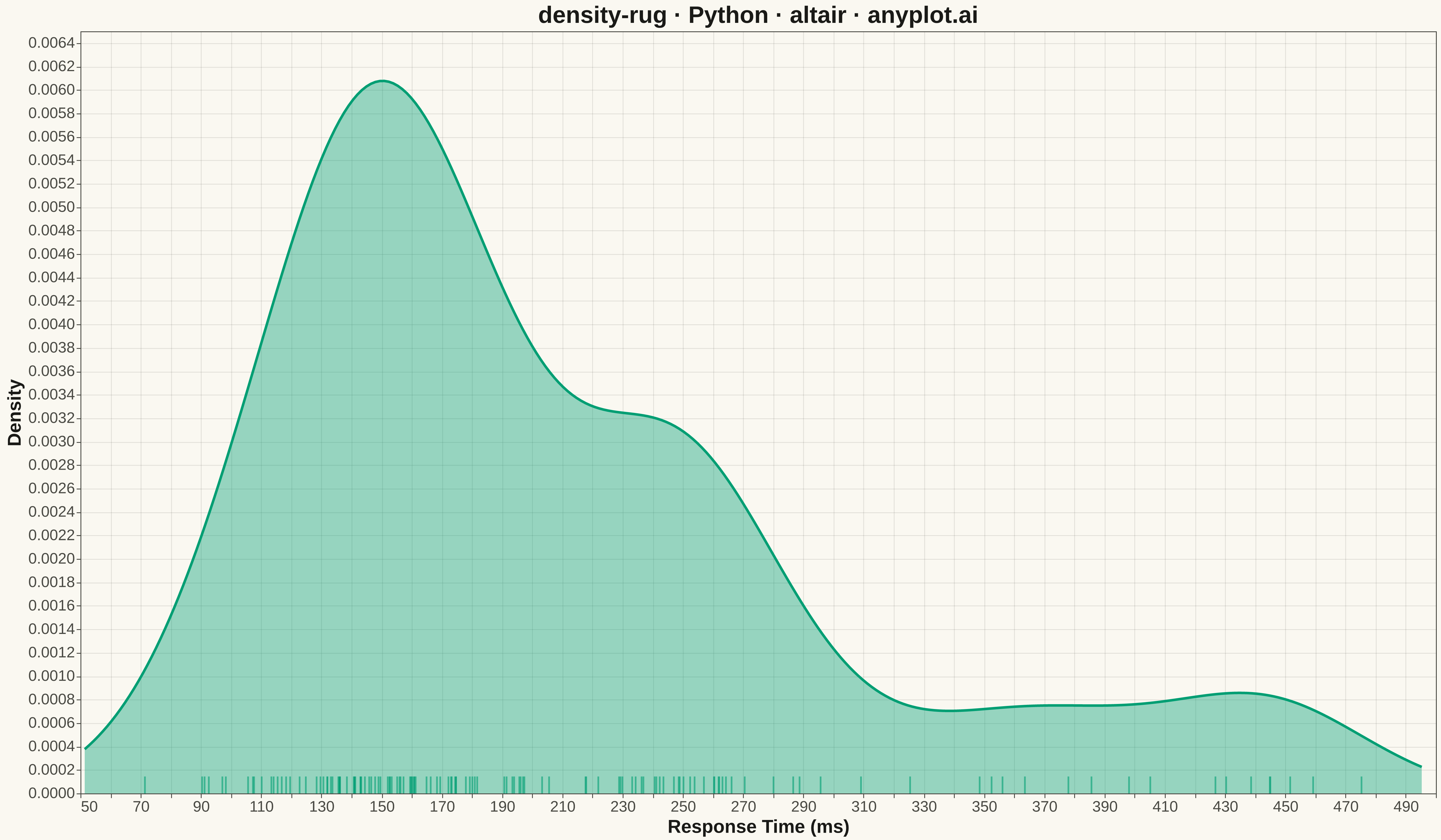
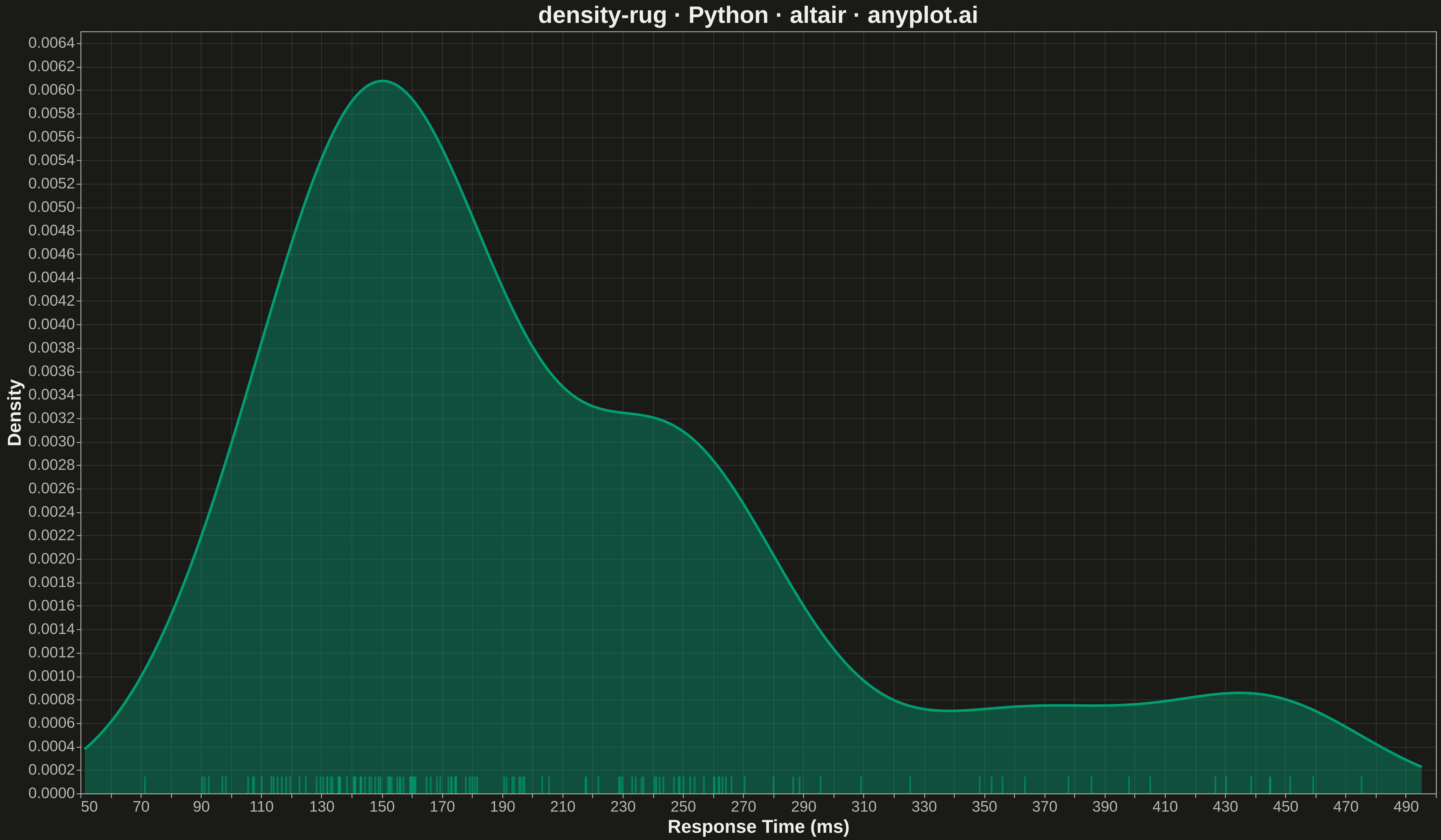
A kernel density estimation (KDE) plot combined with rug marks along the x-axis, showing both the smoothed probability distribution and the exact location of each individual data point. This combination provides the best of both worlds: the KDE reveals the overall shape, modality, and smoothed density of the distribution, while the rug marks preserve transparency about where actual observations fall, highlighting data density and potential gaps.

Density Plot with Rug Marks rendered with Altair

Python source (Altair)

""" anyplot.ai
density-rug: Density Plot with Rug Marks
Library: altair 6.1.0 | Python 3.13.13
Quality: 91/100 | Updated: 2026-05-18
"""

import os
import sys


# Remove current directory from path IMMEDIATELY to avoid import shadowing
if sys.path[0] == "" or sys.path[0] == ".":
    sys.path.pop(0)
# Also remove the script directory if it's there
script_dir = os.path.dirname(os.path.abspath(__file__))
sys.path = [p for p in sys.path if os.path.abspath(p) != script_dir]

import altair as alt
import numpy as np
import pandas as pd
from scipy.stats import gaussian_kde


# Theme tokens
THEME = os.getenv("ANYPLOT_THEME", "light")
PAGE_BG = "#FAF8F1" if THEME == "light" else "#1A1A17"
ELEVATED_BG = "#FFFDF6" if THEME == "light" else "#242420"
INK = "#1A1A17" if THEME == "light" else "#F0EFE8"
INK_SOFT = "#4A4A44" if THEME == "light" else "#B8B7B0"
BRAND = "#009E73"  # Okabe-Ito position 1

# Data - response times (ms) with realistic distribution
np.random.seed(42)
# Mix of normal response times with some slower outliers
response_times = np.concatenate(
    [
        np.random.normal(150, 30, 80),  # Most responses ~150ms
        np.random.normal(250, 40, 40),  # Slower cluster ~250ms
        np.random.uniform(350, 500, 15),  # Some slow outliers
    ]
)
response_times = np.clip(response_times, 50, 500)  # Realistic bounds

# Compute KDE for smooth density curve
kde = gaussian_kde(response_times, bw_method=0.3)
x_range = np.linspace(response_times.min() - 20, response_times.max() + 20, 300)
density_values = kde(x_range)

# Create DataFrames
density_df = pd.DataFrame({"Response Time (ms)": x_range, "Density": density_values})

# For rug marks, add a small y value to position marks above the x-axis
rug_df = pd.DataFrame({"Response Time (ms)": response_times, "rug_y": [0.0] * len(response_times)})

# Density curve with filled area
density_chart = (
    alt.Chart(density_df)
    .mark_area(opacity=0.4, color=BRAND, line={"color": BRAND, "strokeWidth": 3})
    .encode(x=alt.X("Response Time (ms):Q", title="Response Time (ms)"), y=alt.Y("Density:Q", title="Density"))
)

# Rug marks as tick marks along the bottom using a secondary layer
rug_chart = (
    alt.Chart(rug_df)
    .mark_tick(color=BRAND, opacity=0.6, thickness=2, size=40)
    .encode(
        x=alt.X("Response Time (ms):Q"),
        y=alt.Y("rug_y:Q", scale=alt.Scale(domain=[density_values.min(), density_values.max()])),
    )
)

# Combine charts with layering
chart = (
    alt.layer(density_chart, rug_chart)
    .properties(
        width=1600,
        height=900,
        background=PAGE_BG,
        title=alt.Title("density-rug · Python · altair · anyplot.ai", fontSize=28, anchor="middle", color=INK),
    )
    .configure_axis(
        domainColor=INK_SOFT,
        tickColor=INK_SOFT,
        gridColor=INK,
        gridOpacity=0.10,
        labelColor=INK_SOFT,
        titleColor=INK,
        labelFontSize=18,
        titleFontSize=22,
    )
    .configure_view(fill=PAGE_BG, stroke=INK_SOFT, strokeWidth=1)
    .interactive()
)

# Save
chart.save(f"plot-{THEME}.png", scale_factor=3.0)
chart.save(f"plot-{THEME}.html")

Part of Density Plot with Rug Marks on anyplot.ai.

Density Plot with Rug Marks — Altair

Python source (Altair)

Other implementations