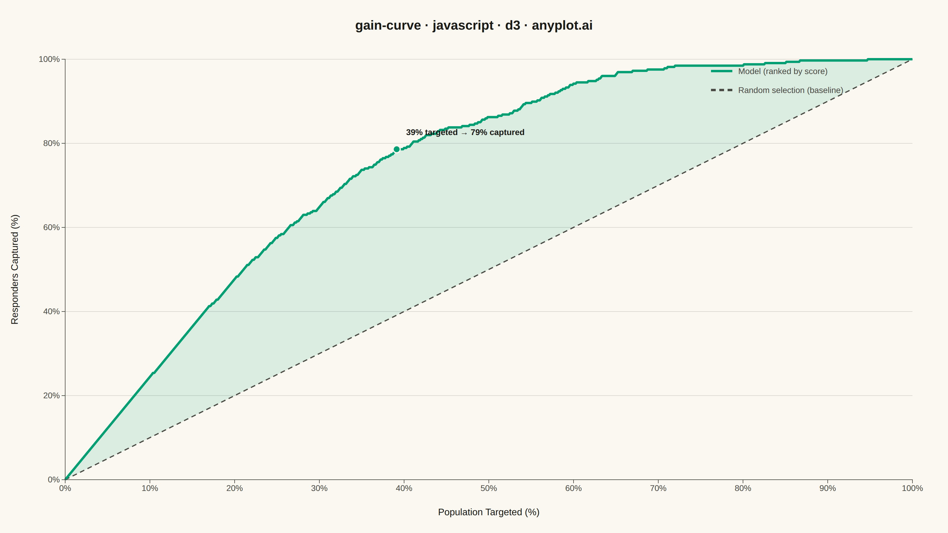
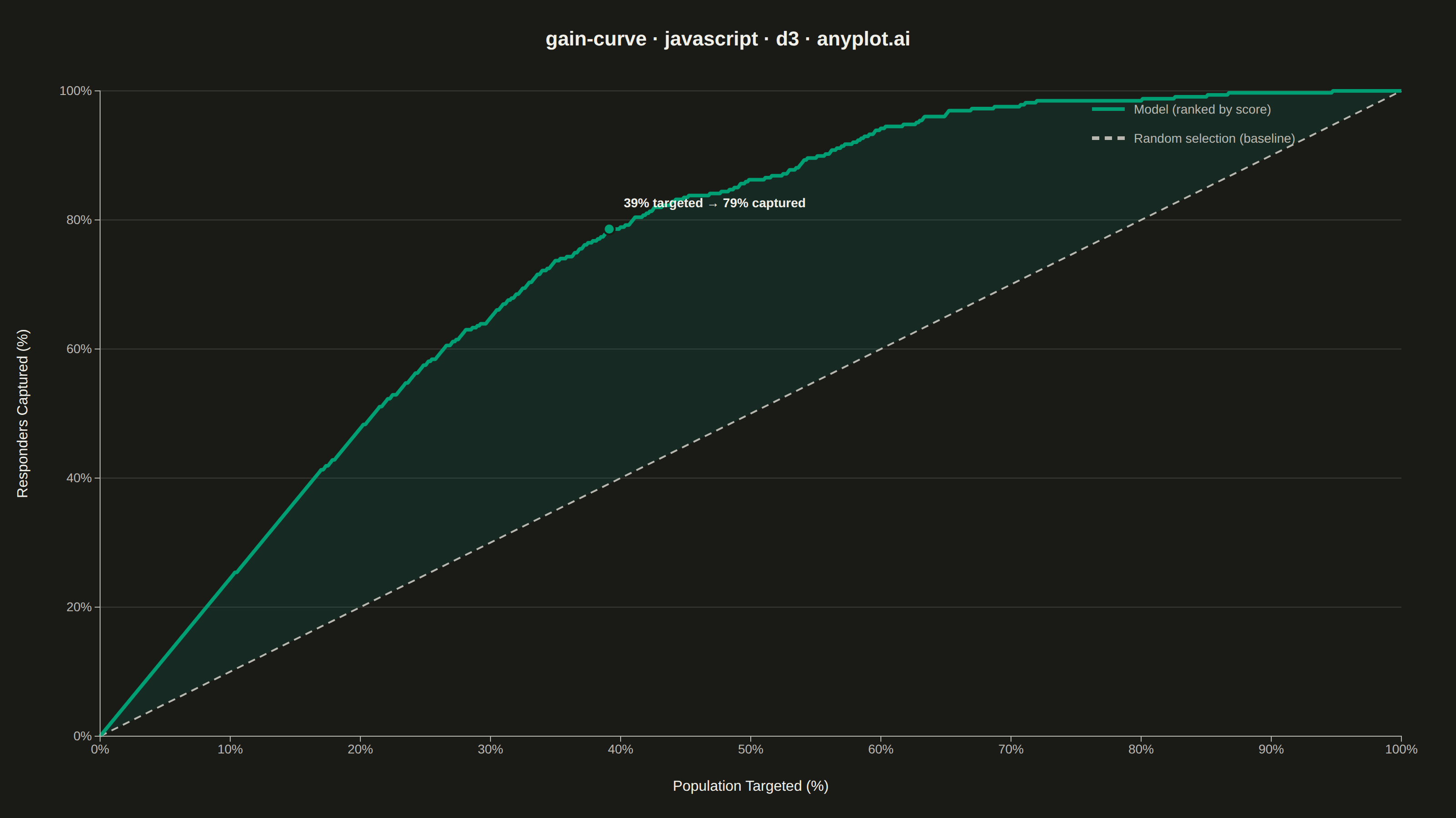
The same plot in 14 other libraries — JavaScript: Chart.js, Apache ECharts, Highcharts, MUI X Charts; Python: Altair, Bokeh, lets-plot, Matplotlib, Plotly, plotnine, Pygal, Seaborn; R: ggplot2; Julia: Makie.jl. Compare all 15 side by side: Cumulative Gains Chart in Python, R, Julia and JavaScript.
A cumulative gains chart visualizes the effectiveness of a classification model by showing what percentage of positive cases is captured when targeting increasing percentages of the population, ranked by predicted probability. It answers the question: "If I target the top X% of my predictions, what percentage of all actual positives will I capture?" This plot is essential for evaluating targeting strategies in marketing, risk assessment, and resource allocation scenarios.
// anyplot.ai
// gain-curve: Cumulative Gains Chart
// Library: d3 7.9.0 | JavaScript 22.23.2
// Quality: 94/100 | Created: 2026-09-05

const t = window.ANYPLOT_TOKENS;
const { width, height } = window.ANYPLOT_SIZE;
const margin = { top: 100, right: 60, bottom: 90, left: 110 };
const iw = width - margin.left - margin.right;
const ih = height - margin.top - margin.bottom;

// --- Data: simulated marketing-campaign response model ----------------------
// Deterministic LCG — the browser has no seeded RNG.
function lcg(seed) {
  let state = seed >>> 0;
  return function () {
    state = (state * 1664525 + 1013904223) >>> 0;
    return state / 4294967296;
  };
}
const rand = lcg(42);

function centeredNoise() {
  return (rand() + rand() + rand() - 1.5) / 1.5; // ~[-1, 1], symmetric around 0
}

const nCustomers = 800;
const customers = [];
for (let i = 0; i < nCustomers; i++) {
  const propensity = Math.pow(rand(), 2.2); // skewed: most customers unlikely to respond
  const responded = rand() < propensity * 1.4 ? 1 : 0;
  const score = Math.min(1, Math.max(0, propensity + centeredNoise() * 0.18));
  customers.push({ responded, score });
}

const rankedByScore = customers.slice().sort((a, b) => b.score - a.score);
const totalResponders = rankedByScore.reduce((sum, c) => sum + c.responded, 0);

const gainCurve = [{ population: 0, captured: 0 }];
let cumulativeResponders = 0;
rankedByScore.forEach((c, i) => {
  cumulativeResponders += c.responded;
  gainCurve.push({
    population: ((i + 1) / nCustomers) * 100,
    captured: (cumulativeResponders / totalResponders) * 100,
  });
});
const baseline = [
  { population: 0, captured: 0 },
  { population: 100, captured: 100 },
];

// Peak-lift point: population % where the model's advantage over random
// selection (captured - population) is greatest.
const peakLift = gainCurve.reduce((best, d) =>
  d.captured - d.population > best.captured - best.population ? d : best
);

// --- SVG mount ----------------------------------------------------------------
const svg = d3.select("#container").append("svg").attr("width", width).attr("height", height);
const g = svg.append("g").attr("transform", `translate(${margin.left},${margin.top})`);

// --- Scales ---------------------------------------------------------------
const x = d3.scaleLinear().domain([0, 100]).range([0, iw]);
const y = d3.scaleLinear().domain([0, 100]).range([ih, 0]);

// --- Gridlines (y-axis only, subtle) ---------------------------------------
g.append("g")
  .selectAll("line")
  .data(y.ticks(5))
  .join("line")
  .attr("x1", 0)
  .attr("x2", iw)
  .attr("y1", (d) => y(d))
  .attr("y2", (d) => y(d))
  .attr("stroke", t.grid);

// --- Gain area (shaded lift over random selection) ---------------------------
// The baseline is the diagonal captured == population, so it can be reused
// directly as the area's lower edge without resampling a second series.
const areaGen = d3
  .area()
  .curve(d3.curveMonotoneX)
  .x((d) => x(d.population))
  .y0((d) => y(d.population))
  .y1((d) => y(d.captured));

g.append("path")
  .datum(gainCurve)
  .attr("fill", t.palette[0])
  .attr("fill-opacity", 0.12)
  .attr("d", areaGen);

// --- Baseline (random-selection reference) ----------------------------------
const lineGen = d3
  .line()
  .curve(d3.curveMonotoneX)
  .x((d) => x(d.population))
  .y((d) => y(d.captured));

g.append("path")
  .datum(baseline)
  .attr("fill", "none")
  .attr("stroke", t.inkSoft)
  .attr("stroke-width", 2)
  .attr("stroke-dasharray", "8,6")
  .attr("d", lineGen);

// --- Model gain curve --------------------------------------------------------
g.append("path")
  .datum(gainCurve)
  .attr("fill", "none")
  .attr("stroke", t.palette[0])
  .attr("stroke-width", 4)
  .attr("stroke-linejoin", "round")
  .attr("d", lineGen);

// --- Peak-lift annotation -----------------------------------------------------
g.append("circle")
  .attr("cx", x(peakLift.population))
  .attr("cy", y(peakLift.captured))
  .attr("r", 6)
  .attr("fill", t.palette[0])
  .attr("stroke", t.pageBg)
  .attr("stroke-width", 2);

const callout = g
  .append("g")
  .attr("transform", `translate(${x(peakLift.population) + 16}, ${y(peakLift.captured) - 24})`);
callout
  .append("text")
  .attr("fill", t.ink)
  .style("font-size", "14px")
  .style("font-weight", "600")
  .text(`${peakLift.population.toFixed(0)}% targeted → ${peakLift.captured.toFixed(0)}% captured`);

// --- Axes -------------------------------------------------------------------
const xAxis = g
  .append("g")
  .attr("transform", `translate(0,${ih})`)
  .call(d3.axisBottom(x).ticks(10).tickFormat((d) => `${d}%`));
const yAxis = g.append("g").call(d3.axisLeft(y).ticks(5).tickFormat((d) => `${d}%`));

for (const axis of [xAxis, yAxis]) {
  axis.selectAll("text").attr("fill", t.inkSoft).style("font-size", "14px");
  axis.selectAll("line").attr("stroke", t.inkSoft);
  axis.select(".domain").attr("stroke", t.inkSoft);
}
g.selectAll(".tick line").attr("stroke", t.inkSoft);

// --- Axis labels --------------------------------------------------------------
g.append("text")
  .attr("x", iw / 2)
  .attr("y", ih + 60)
  .attr("text-anchor", "middle")
  .attr("fill", t.ink)
  .style("font-size", "16px")
  .text("Population Targeted (%)");

g.append("text")
  .attr("transform", "rotate(-90)")
  .attr("x", -ih / 2)
  .attr("y", -80)
  .attr("text-anchor", "middle")
  .attr("fill", t.ink)
  .style("font-size", "16px")
  .text("Responders Captured (%)");

// --- Legend -------------------------------------------------------------------
const legend = g.append("g").attr("transform", `translate(${iw - 340}, 20)`);
const legendItems = [
  { label: "Model (ranked by score)", color: t.palette[0], dashed: false },
  { label: "Random selection (baseline)", color: t.inkSoft, dashed: true },
];
legendItems.forEach((item, i) => {
  const row = legend.append("g").attr("transform", `translate(0, ${i * 32})`);
  row
    .append("line")
    .attr("x1", 0)
    .attr("x2", 36)
    .attr("y1", 0)
    .attr("y2", 0)
    .attr("stroke", item.color)
    .attr("stroke-width", 4)
    .attr("stroke-dasharray", item.dashed ? "8,6" : null);
  row
    .append("text")
    .attr("x", 46)
    .attr("y", 5)
    .attr("fill", t.inkSoft)
    .style("font-size", "14px")
    .text(item.label);
});

// --- Title --------------------------------------------------------------------
svg
  .append("text")
  .attr("x", width / 2)
  .attr("y", 50)
  .attr("text-anchor", "middle")
  .attr("fill", t.ink)
  .style("font-size", "22px")
  .style("font-weight", "600")
  .text("gain-curve · javascript · d3 · anyplot.ai");
Runnable source as JSON, for any HTTP client: https://api.anyplot.ai/specs/gain-curve/d3/code. Any spec id and library id listed in llms-full.txt fit the same URL shape; every URL below is complete and callable.
{
  "spec_id": "gain-curve",
  "language": "javascript",
  "library": "d3",
  "page": "https://anyplot.ai/gain-curve/javascript/d3",
  "hub": "https://anyplot.ai/gain-curve",
  "code_json": "https://api.anyplot.ai/specs/gain-curve/d3/code",
  "spec_json": "https://api.anyplot.ai/specs/gain-curve",
  "render_light_png": "https://storage.googleapis.com/anyplot-images/plots/gain-curve/javascript/d3/plot-light.png",
  "render_dark_png": "https://storage.googleapis.com/anyplot-images/plots/gain-curve/javascript/d3/plot-dark.png",
  "interactive_light_html": "https://storage.googleapis.com/anyplot-images/plots/gain-curve/javascript/d3/plot-light.html",
  "interactive_dark_html": "https://storage.googleapis.com/anyplot-images/plots/gain-curve/javascript/d3/plot-dark.html",
  "quality_score": 94.0,
  "license": "MIT",
  "guide": "https://anyplot.ai/llms.txt"
}
Part of Cumulative Gains Chart on anyplot.ai.