The same plot in 14 other libraries — Python: Altair, Bokeh, lets-plot, Matplotlib, Plotly, plotnine, Pygal, Seaborn; Julia: Makie.jl; JavaScript: Chart.js, D3.js, Apache ECharts, Highcharts, MUI X Charts. Compare all 15 side by side: Training Loss Curve in Python, R, Julia and JavaScript.
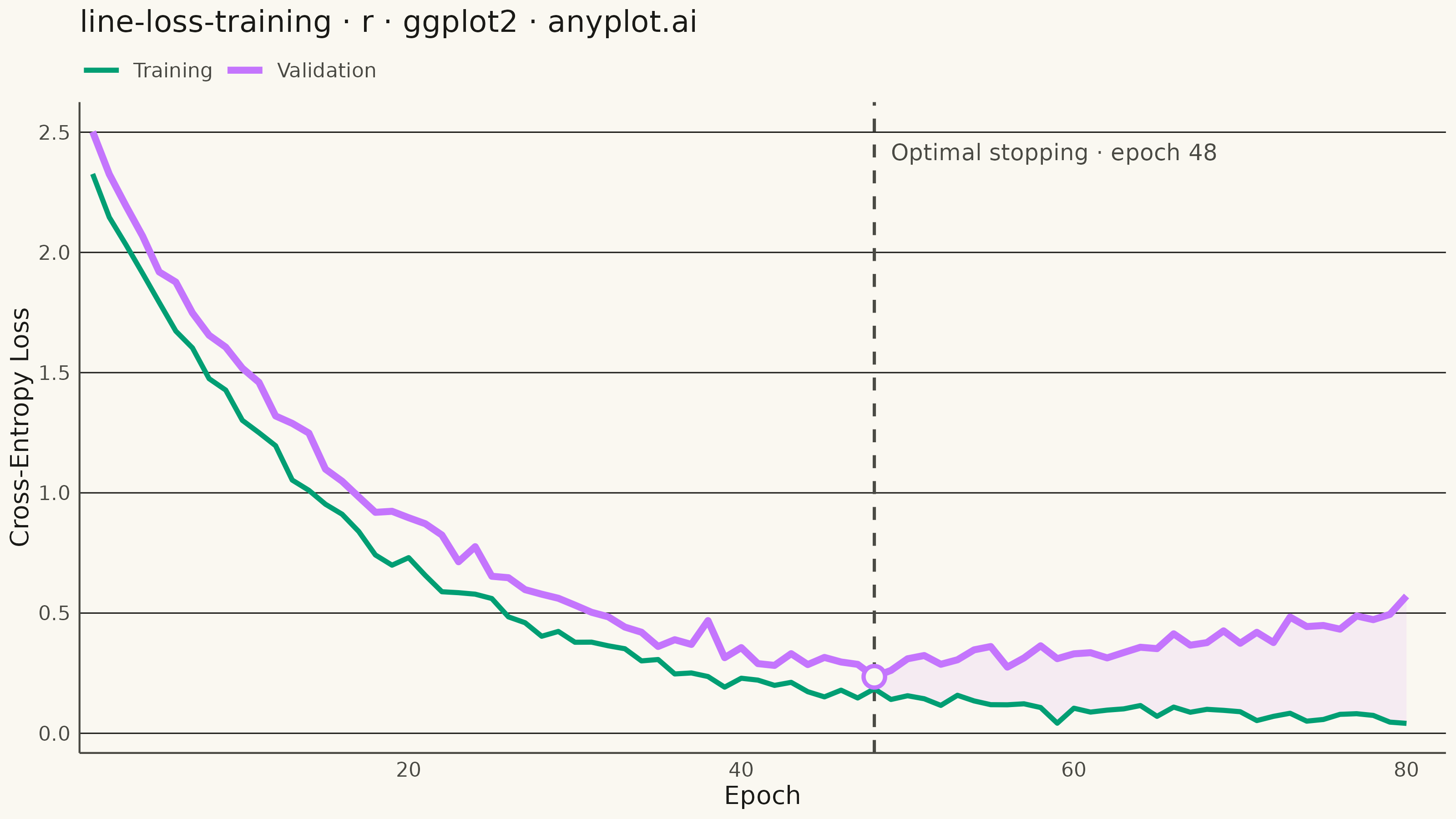
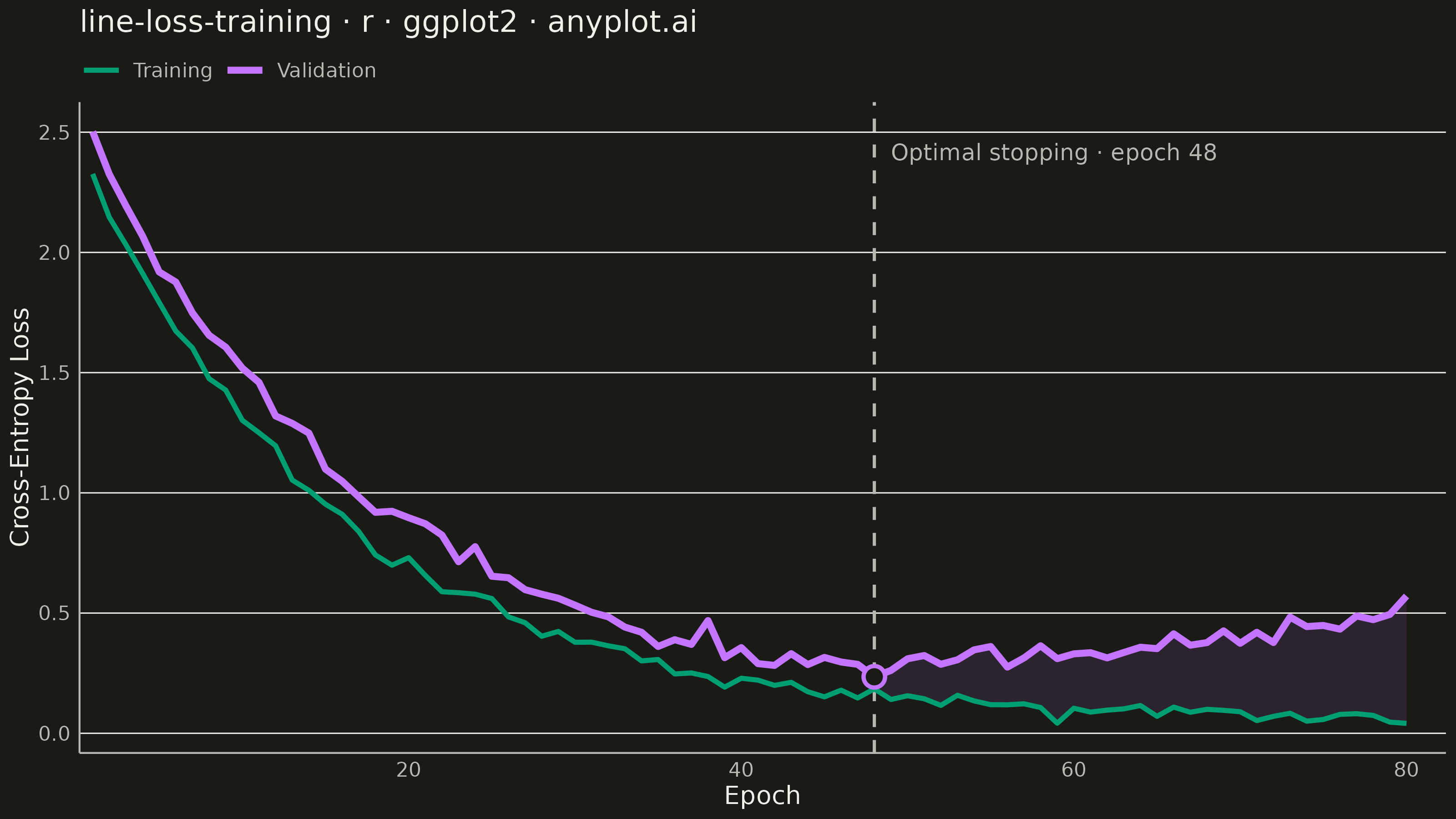
A line plot showing training and validation loss curves over epochs during neural network training. This visualization is essential for monitoring model training, detecting overfitting (when validation loss diverges from training loss), and determining optimal early stopping points. The dual-curve display reveals the gap between training and generalization performance.
#' anyplot.ai
#' line-loss-training: Training Loss Curve
#' Library: ggplot2 3.5.1 | R 4.4.1
#' Quality: 91/100 | Created: 2026-09-05

library(ggplot2)
library(dplyr)
library(tidyr)
library(ragg)

set.seed(42)

# --- Theme tokens ------------------------------------------------------------
THEME       <- Sys.getenv("ANYPLOT_THEME", "light")
PAGE_BG     <- if (THEME == "light") "#FAF8F1" else "#1A1A17"
INK         <- if (THEME == "light") "#1A1A17" else "#F0EFE8"
INK_SOFT    <- if (THEME == "light") "#4A4A44" else "#B8B7B0"

# Imprint palette — canonical order (position 1 always brand green)
IMPRINT_PALETTE <- c(
  "#009E73", # 1 — training loss
  "#C475FD"  # 2 — validation loss
)

# --- Data --------------------------------------------------------------------
# Simulated training history for an image classifier trained for 80 epochs.
# Training loss decays smoothly; validation loss decays then climbs again
# past epoch ~34, the classic overfitting signature.
n_epochs <- 80
epoch <- 1:n_epochs

train_loss <- 2.4 * exp(-epoch * 0.065) + 0.05 + rnorm(n_epochs, 0, 0.02)
train_loss <- pmax(train_loss, 0.02)

overfit_penalty <- 0.0009 * pmax(0, epoch - 34)^1.6
val_loss <- 2.5 * exp(-epoch * 0.058) + 0.09 + overfit_penalty + rnorm(n_epochs, 0, 0.035)
val_loss <- pmax(val_loss, 0.05)

history_wide <- tibble::tibble(epoch, train_loss, val_loss)
history <- history_wide |>
  pivot_longer(cols = c(train_loss, val_loss), names_to = "split", values_to = "loss") |>
  mutate(split = factor(split,
    levels = c("train_loss", "val_loss"),
    labels = c("Training", "Validation")
  ))

best_epoch <- epoch[which.min(val_loss)]
best_val_loss <- min(val_loss)

# Generalization-gap ribbon: shade the area between the curves once
# validation loss has diverged past the optimal-stopping epoch.
gap_region <- history_wide |> filter(epoch >= best_epoch)

# --- Plot ----------------------------------------------------------------
p <- ggplot(history, aes(x = epoch, y = loss, color = split, linewidth = split)) +
  geom_ribbon(
    data = gap_region,
    aes(x = epoch, ymin = train_loss, ymax = val_loss),
    inherit.aes = FALSE,
    fill = IMPRINT_PALETTE[2], alpha = 0.10
  ) +
  geom_vline(xintercept = best_epoch, linetype = "dashed", linewidth = 0.6, color = INK_SOFT) +
  geom_line() +
  annotate("point",
    x = best_epoch, y = best_val_loss,
    color = IMPRINT_PALETTE[2], size = 3.2, shape = 21, fill = PAGE_BG, stroke = 1.2
  ) +
  annotate("text",
    x = best_epoch, y = max(train_loss, val_loss) * 0.98,
    label = sprintf("Optimal stopping · epoch %d", best_epoch),
    color = INK_SOFT, size = 3.2, hjust = -0.05, vjust = 1
  ) +
  scale_color_manual(values = IMPRINT_PALETTE) +
  scale_linewidth_manual(values = c(Training = 0.95, Validation = 1.3)) +
  scale_x_continuous(expand = expansion(mult = c(0.01, 0.03))) +
  labs(
    title = "line-loss-training · r · ggplot2 · anyplot.ai",
    x = "Epoch",
    y = "Cross-Entropy Loss",
    color = NULL,
    linewidth = NULL
  ) +
  theme_minimal(base_size = 8) +
  theme(
    plot.background   = element_rect(fill = PAGE_BG, color = PAGE_BG),
    panel.background  = element_rect(fill = PAGE_BG, color = NA),
    panel.grid.major  = element_line(color = INK, linewidth = 0.25),
    panel.grid.minor  = element_blank(),
    panel.grid.major.x = element_blank(),
    axis.title        = element_text(color = INK, size = 10),
    axis.text         = element_text(color = INK_SOFT, size = 8),
    axis.line         = element_line(color = INK_SOFT),
    plot.title        = element_text(color = INK, size = 12),
    legend.position    = "top",
    legend.justification = "left",
    legend.margin      = margin(t = 0, b = -4, l = 0, r = 0),
    legend.background  = element_blank(),
    legend.key         = element_blank(),
    legend.text        = element_text(color = INK_SOFT, size = 8),
    legend.title       = element_text(color = INK, size = 10)
  )

# --- Save --------------------------------------------------------------------
ggsave(
  filename = sprintf("plot-%s.png", THEME),
  plot     = p,
  device   = ragg::agg_png,
  width    = 8,
  height   = 4.5,
  units    = "in",
  dpi      = 400
)
Runnable source as JSON, for any HTTP client: https://api.anyplot.ai/specs/line-loss-training/ggplot2/code. Any spec id and library id listed in llms-full.txt fit the same URL shape; every URL below is complete and callable.
{
  "spec_id": "line-loss-training",
  "language": "r",
  "library": "ggplot2",
  "page": "https://anyplot.ai/line-loss-training/r/ggplot2",
  "hub": "https://anyplot.ai/line-loss-training",
  "code_json": "https://api.anyplot.ai/specs/line-loss-training/ggplot2/code",
  "spec_json": "https://api.anyplot.ai/specs/line-loss-training",
  "render_light_png": "https://storage.googleapis.com/anyplot-images/plots/line-loss-training/r/ggplot2/plot-light.png",
  "render_dark_png": "https://storage.googleapis.com/anyplot-images/plots/line-loss-training/r/ggplot2/plot-dark.png",
  "quality_score": 91.0,
  "license": "MIT",
  "guide": "https://anyplot.ai/llms.txt"
}
Part of Training Loss Curve on anyplot.ai.