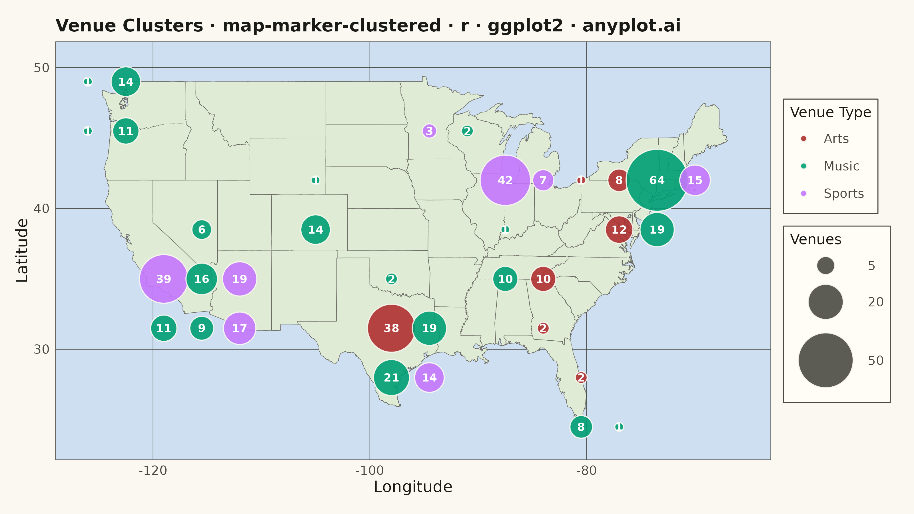
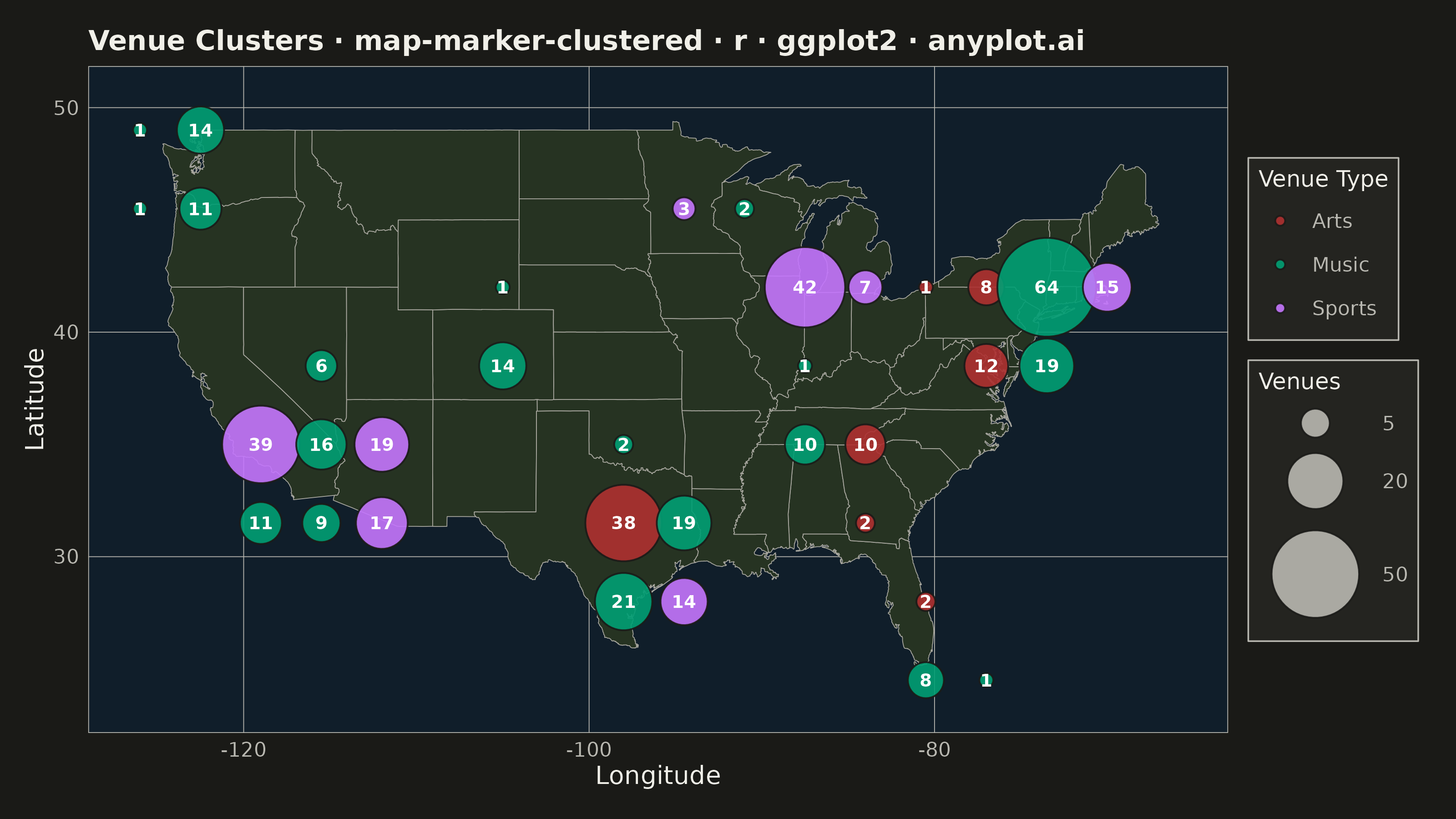
The same plot in 14 other libraries — Python: Altair, Bokeh, lets-plot, Matplotlib, Plotly, plotnine, Pygal, Seaborn; Julia: Makie.jl; JavaScript: Chart.js, D3.js, Apache ECharts, Highcharts, MUI X Charts. Compare all 15 side by side: Clustered Marker Map in Python, R, Julia and JavaScript.
A geographic map that dynamically clusters nearby markers based on the current zoom level. At lower zoom levels, clusters aggregate multiple points into a single marker displaying the count, while zooming in progressively expands clusters to reveal individual markers. This visualization is essential for efficiently displaying large geographic datasets without visual clutter, enabling users to see both the overall distribution and specific locations through interactive exploration.
#' anyplot.ai
#' map-marker-clustered: Clustered Marker Map
#' Library: ggplot2 3.5.1 | R 4.4.1
#' Quality: 85/100 | Created: 2026-05-23

library(ggplot2)
library(dplyr)
library(ragg)

set.seed(42)

# --- Theme tokens -----------------------------------------------------------
THEME       <- Sys.getenv("ANYPLOT_THEME", "light")
PAGE_BG     <- if (THEME == "light") "#FAF8F1" else "#1A1A17"
ELEVATED_BG <- if (THEME == "light") "#FFFDF6" else "#242420"
INK         <- if (THEME == "light") "#1A1A17" else "#F0EFE8"
INK_SOFT    <- if (THEME == "light") "#4A4A44" else "#B8B7B0"
INK_MUTED   <- if (THEME == "light") "#6B6A63" else "#A8A79F"
WATER_BG    <- if (THEME == "light") "#CDDFF0" else "#101E2A"
LAND_FILL   <- if (THEME == "light") "#E0EBD5" else "#263322"

IMPRINT <- c(
    "#009E73",  # 1: Music venues
    "#C475FD",  # 2: Sports venues
    "#AE3030"   # 3: Arts venues
)
categories <- c("Music", "Sports", "Arts")

# --- Data -------------------------------------------------------------------
metro_areas <- data.frame(
    lat = c(
        40.71, 34.05, 41.88, 29.76, 33.45, 39.95, 29.42,
        32.72, 32.78, 30.27, 47.61, 39.74, 42.36, 25.77,
        45.52, 44.98, 33.75, 42.33, 36.17, 36.16
    ),
    lon = c(
        -74.01, -118.24, -87.63, -95.37, -112.07, -75.17, -98.49,
        -117.16, -96.80, -97.74, -122.33, -104.99, -71.06, -80.19,
        -122.68, -93.27, -84.39, -83.05, -115.14, -86.78
    ),
    weight = c(15, 12, 10, 7, 7, 6, 5, 5, 5, 5, 4, 4, 4, 3, 3, 2, 2, 2, 2, 2)
)

n_venues <- 460
city_idx <- sample(
    nrow(metro_areas), n_venues,
    replace = TRUE,
    prob    = metro_areas$weight / sum(metro_areas$weight)
)

venues <- data.frame(
    lat      = metro_areas$lat[city_idx] + rnorm(n_venues, 0, 0.55),
    lon      = metro_areas$lon[city_idx] + rnorm(n_venues, 0, 0.75),
    category = sample(categories, n_venues, replace = TRUE, prob = c(0.40, 0.35, 0.25))
)

# Grid-based pre-clustering — simulates a fixed zoom-level snapshot
grid_res <- 3.5
clusters <- venues %>%
    mutate(
        clat = round(lat / grid_res) * grid_res,
        clon = round(lon / grid_res) * grid_res
    ) %>%
    group_by(clat, clon) %>%
    summarize(
        count    = dplyr::n(),
        category = names(sort(table(category), decreasing = TRUE))[1],
        .groups  = "drop"
    )

us_states <- map_data("state")

# --- Plot -------------------------------------------------------------------
p <- ggplot() +
    geom_polygon(
        data      = us_states,
        aes(x = long, y = lat, group = group),
        fill      = LAND_FILL,
        color     = INK_MUTED,
        linewidth = 0.15
    ) +
    geom_point(
        data   = clusters,
        aes(x = clon, y = clat, size = count, fill = category),
        shape  = 21,
        color  = PAGE_BG,
        alpha  = 0.90,
        stroke = 0.5
    ) +
    geom_text(
        data     = clusters,
        aes(x = clon, y = clat, label = count),
        size     = 2.5,
        color    = "white",
        fontface = "bold"
    ) +
    scale_fill_manual(
        values = setNames(IMPRINT, categories),
        name   = "Venue Type"
    ) +
    scale_size_area(
        max_size = 18,
        name     = "Venues",
        breaks   = c(5, 20, 50, 80),
        guide    = guide_legend(
            override.aes = list(fill = INK_SOFT, color = PAGE_BG, stroke = 0.5)
        )
    ) +
    coord_fixed(
        ratio = 1.3,
        xlim  = c(-126, -66),
        ylim  = c(23.5, 50.5)
    ) +
    labs(
        title = "Venue Clusters · map-marker-clustered · r · ggplot2 · anyplot.ai",
        x     = "Longitude",
        y     = "Latitude"
    ) +
    theme_minimal(base_size = 8) +
    theme(
        plot.background   = element_rect(fill = PAGE_BG, color = PAGE_BG),
        panel.background  = element_rect(fill = WATER_BG, color = NA),
        panel.grid.major  = element_line(color = INK_SOFT, linewidth = 0.15),
        panel.grid.minor  = element_blank(),
        panel.border      = element_rect(fill = NA, color = INK_SOFT, linewidth = 0.3),
        axis.title        = element_text(color = INK, size = 10),
        axis.text         = element_text(color = INK_SOFT, size = 8),
        plot.title        = element_text(color = INK, size = 11, face = "bold"),
        legend.background = element_rect(fill = ELEVATED_BG, color = INK_SOFT, linewidth = 0.3),
        legend.text       = element_text(color = INK_SOFT, size = 8),
        legend.title      = element_text(color = INK, size = 9),
        legend.key        = element_rect(fill = NA, color = NA),
        plot.margin       = margin(10, 15, 10, 10)
    )

# --- Save -------------------------------------------------------------------
ggsave(
    filename = sprintf("plot-%s.png", THEME),
    plot     = p,
    device   = ragg::agg_png,
    width    = 8,
    height   = 4.5,
    units    = "in",
    dpi      = 400
)
Runnable source as JSON, for any HTTP client: https://api.anyplot.ai/specs/map-marker-clustered/ggplot2/code. Any spec id and library id listed in llms-full.txt fit the same URL shape; every URL below is complete and callable.
{
  "spec_id": "map-marker-clustered",
  "language": "r",
  "library": "ggplot2",
  "page": "https://anyplot.ai/map-marker-clustered/r/ggplot2",
  "hub": "https://anyplot.ai/map-marker-clustered",
  "code_json": "https://api.anyplot.ai/specs/map-marker-clustered/ggplot2/code",
  "spec_json": "https://api.anyplot.ai/specs/map-marker-clustered",
  "render_light_png": "https://storage.googleapis.com/anyplot-images/plots/map-marker-clustered/r/ggplot2/plot-light.png",
  "render_dark_png": "https://storage.googleapis.com/anyplot-images/plots/map-marker-clustered/r/ggplot2/plot-dark.png",
  "quality_score": 85.0,
  "license": "MIT",
  "guide": "https://anyplot.ai/llms.txt"
}
Part of Clustered Marker Map on anyplot.ai.