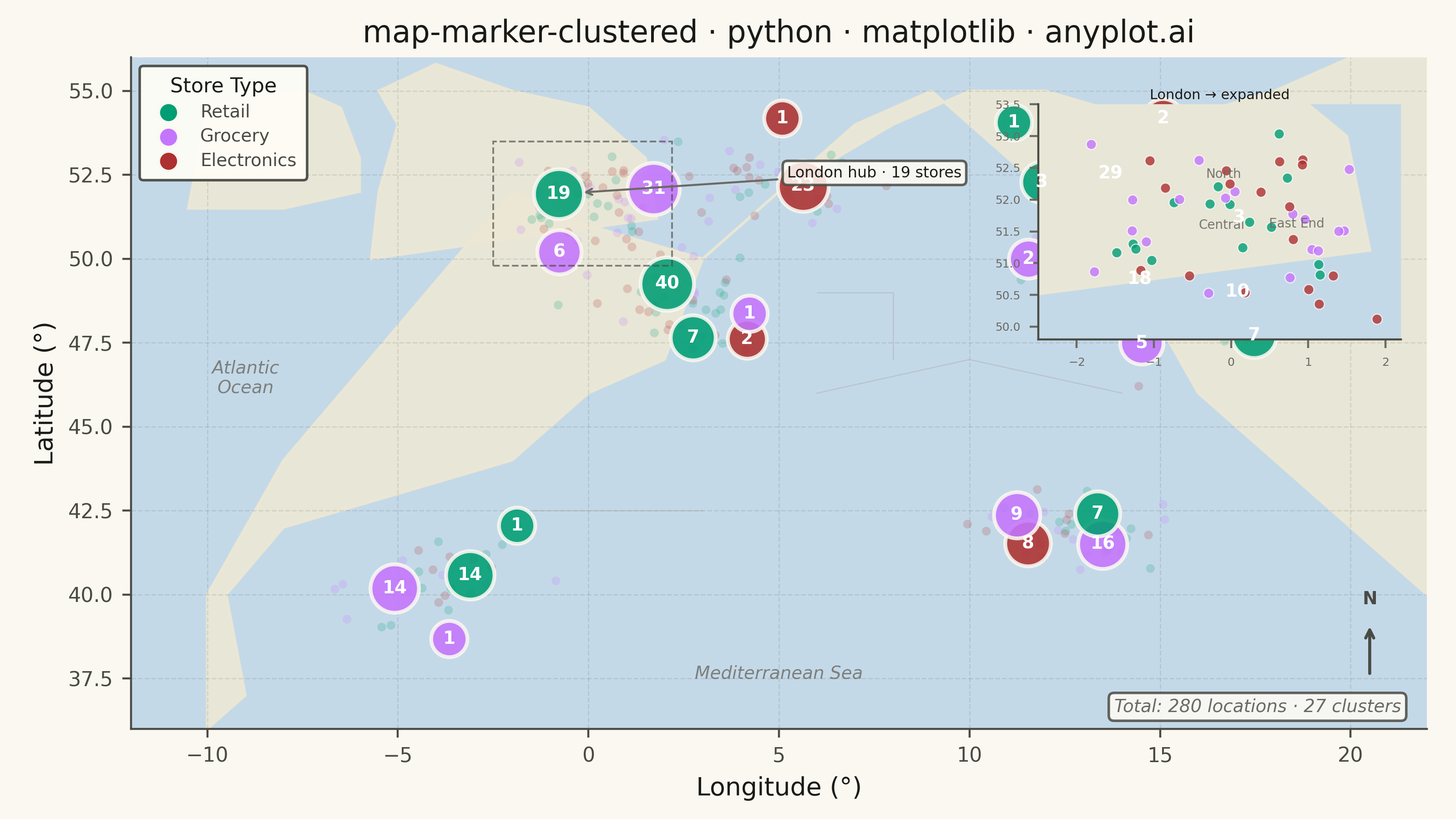
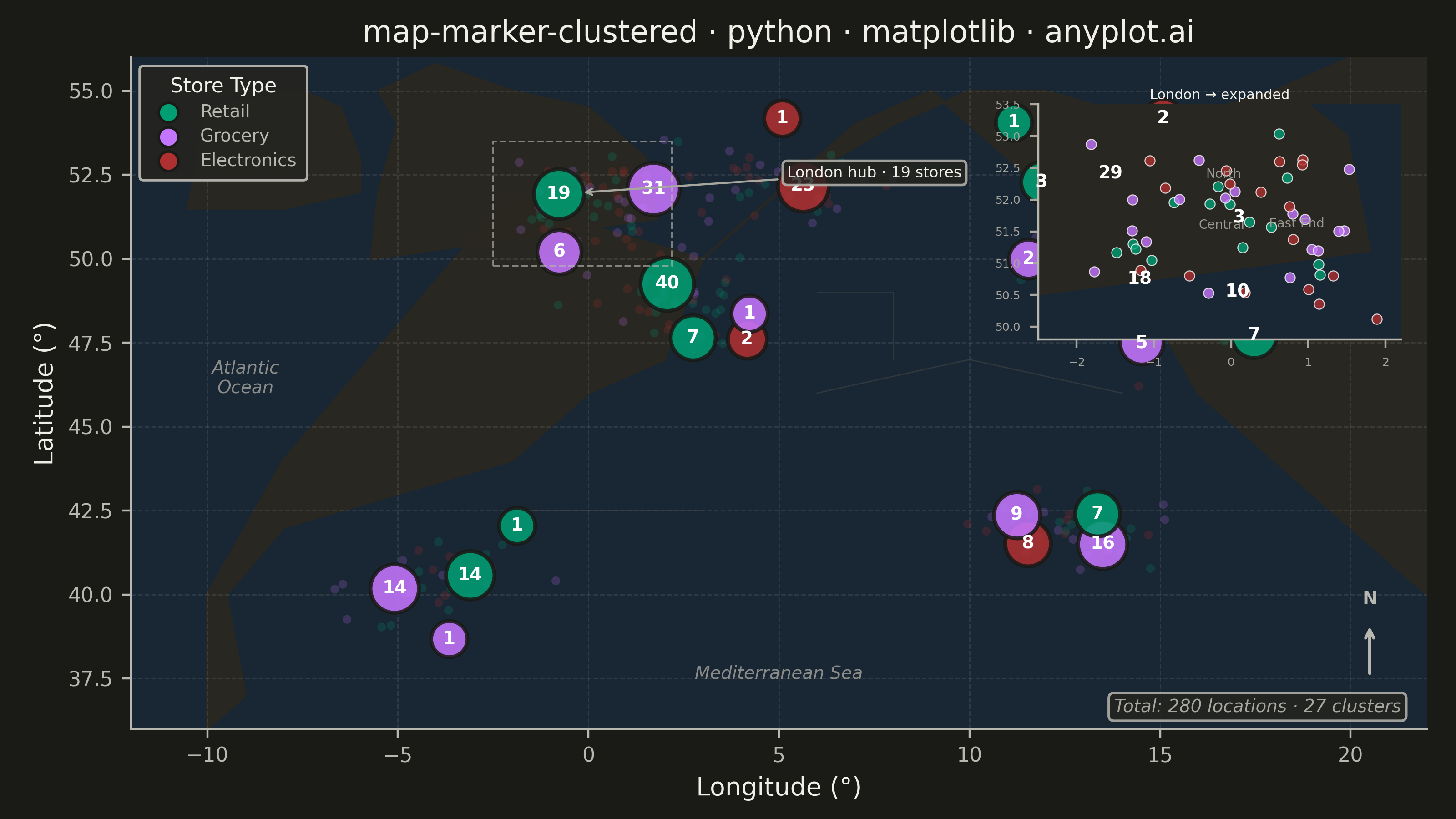
A geographic map that dynamically clusters nearby markers based on the current zoom level. At lower zoom levels, clusters aggregate multiple points into a single marker displaying the count, while zooming in progressively expands clusters to reveal individual markers. This visualization is essential for efficiently displaying large geographic datasets without visual clutter, enabling users to see both the overall distribution and specific locations through interactive exploration.
""" anyplot.ai
map-marker-clustered: Clustered Marker Map
Library: matplotlib 3.10.9 | Python 3.13.13
Quality: 90/100 | Updated: 2026-05-23
"""

import os

import matplotlib.pyplot as plt
import numpy as np
from matplotlib.patches import FancyArrowPatch, Rectangle


# Theme tokens
THEME = os.getenv("ANYPLOT_THEME", "light")
PAGE_BG = "#FAF8F1" if THEME == "light" else "#1A1A17"
ELEVATED_BG = "#FFFDF6" if THEME == "light" else "#242420"
INK = "#1A1A17" if THEME == "light" else "#F0EFE8"
INK_SOFT = "#4A4A44" if THEME == "light" else "#B8B7B0"
INK_MUTED = "#6B6A63" if THEME == "light" else "#A8A79F"

# Geographic context colors (theme-adaptive)
OCEAN_BG = "#C4D9E8" if THEME == "light" else "#192633"
LAND_BG = "#EDE8D4" if THEME == "light" else "#2A2820"
BORDER_COL = "#AAAAAA" if THEME == "light" else "#555550"

# anyplot categorical palette (positions 1-3)
cat_names = ["Retail", "Grocery", "Electronics"]
cat_colors = {"Retail": "#009E73", "Grocery": "#C475FD", "Electronics": "#AE3030"}

# Data: European store locations clustered by city
np.random.seed(42)
city_centers = [
    (48.8566, 2.3522),  # Paris
    (51.5074, -0.1278),  # London
    (52.5200, 13.4050),  # Berlin
    (41.9028, 12.4964),  # Rome
    (40.4168, -3.7038),  # Madrid
    (48.2082, 16.3738),  # Vienna
    (50.0755, 14.4378),  # Prague
    (52.3676, 4.9041),  # Amsterdam
]
n_points_per_city = [45, 50, 35, 40, 30, 25, 20, 35]

lats, lons, categories = [], [], []
for (lat, lon), n_points in zip(city_centers, n_points_per_city, strict=True):
    lats.extend(np.random.normal(lat, 0.8, n_points))
    lons.extend(np.random.normal(lon, 1.2, n_points))
    categories.extend(np.random.choice(cat_names, n_points))

lats = np.array(lats)
lons = np.array(lons)
categories = np.array(categories)

# Grid-based clustering (simulates zoom-level clustering)
grid_size_lat = 3.0
grid_size_lon = 4.0
lat_bins = np.floor((lats - 36) / grid_size_lat).astype(int)
lon_bins = np.floor((lons + 12) / grid_size_lon).astype(int)
cell_ids = lat_bins * 100 + lon_bins

cluster_centers, cluster_sizes, cluster_dominant_cat = [], [], []
for cell_id in np.unique(cell_ids):
    mask = cell_ids == cell_id
    cluster_cats = categories[mask]
    unique_cats, counts = np.unique(cluster_cats, return_counts=True)
    cluster_centers.append((np.mean(lats[mask]), np.mean(lons[mask])))
    cluster_sizes.append(int(np.sum(mask)))
    cluster_dominant_cat.append(unique_cats[np.argmax(counts)])

cluster_centers = np.array(cluster_centers)
cluster_sizes = np.array(cluster_sizes)
cluster_dominant_cat = np.array(cluster_dominant_cat)

# Plot
fig, ax = plt.subplots(figsize=(8, 4.5), dpi=400, facecolor=PAGE_BG)
ax.set_facecolor(OCEAN_BG)

# Simplified European land polygon
europe_coast_lon = [
    -10,
    -9,
    -9.5,
    -8,
    -5,
    -2,
    0,
    2,
    3,
    5,
    7,
    9,
    10,
    12,
    13,
    15,
    16,
    18,
    20,
    22,
    22,
    20,
    18,
    15,
    12,
    10,
    8,
    5,
    3,
    0,
    -2,
    -5,
    -8,
    -10,
    -10,
]
europe_coast_lat = [
    36,
    37,
    40,
    42,
    43,
    44,
    46,
    47,
    50,
    52,
    54,
    55,
    54,
    52,
    50,
    48,
    46,
    44,
    42,
    40,
    56,
    56,
    55,
    54,
    55,
    55,
    54,
    52,
    50,
    51,
    52,
    48,
    44,
    40,
    36,
]
ax.fill(europe_coast_lon, europe_coast_lat, color=LAND_BG, alpha=0.9, zorder=1)

# British Isles — Great Britain and Ireland (fills the map's western extent)
gb_lon = [-5.7, 1.8, 1.5, 0.0, -2.0, -4.0, -5.5, -5.0, -5.5, -5.7]
gb_lat = [50.0, 51.2, 53.0, 54.5, 55.0, 55.8, 55.0, 54.0, 52.0, 50.0]
ax.fill(gb_lon, gb_lat, color=LAND_BG, alpha=0.9, zorder=1)

ie_lon = [-10.5, -8.0, -6.0, -6.0, -6.5, -7.5, -10.0, -10.5]
ie_lat = [51.5, 51.5, 52.0, 53.0, 54.5, 55.0, 54.5, 51.5]
ax.fill(ie_lon, ie_lat, color=LAND_BG, alpha=0.9, zorder=1)

# Country boundary lines
ax.plot([-2, 3], [42.5, 42.5], color=BORDER_COL, linewidth=0.5, alpha=0.4, zorder=2)
ax.plot([6, 8, 8], [49, 49, 47], color=BORDER_COL, linewidth=0.5, alpha=0.4, zorder=2)
ax.plot([15, 15], [51, 54], color=BORDER_COL, linewidth=0.5, alpha=0.4, zorder=2)
ax.plot([6, 10, 14], [46, 47, 46], color=BORDER_COL, linewidth=0.5, alpha=0.4, zorder=2)

# Subtle coordinate grid
ax.grid(True, alpha=0.10, linestyle="--", color=INK, linewidth=0.5, zorder=3)

# Individual data points (semi-transparent density backdrop)
for cat in cat_names:
    mask = categories == cat
    ax.scatter(lons[mask], lats[mask], c=cat_colors[cat], alpha=0.20, s=12, edgecolors="none", zorder=4)

# Cluster markers — logarithmic size scaling prevents over-large small-count markers
for center, size, cat in zip(cluster_centers, cluster_sizes, cluster_dominant_cat, strict=True):
    lat, lon = center
    marker_size = 150 + np.log1p(size) * 80
    ax.scatter(lon, lat, s=marker_size, c=cat_colors[cat], alpha=0.88, edgecolors=PAGE_BG, linewidths=1.5, zorder=5)
    ax.annotate(str(size), (lon, lat), fontsize=7, fontweight="bold", ha="center", va="center", color="white", zorder=6)

# Data storytelling: annotate the London cluster (highest-count city) as the key insight
london_ref_lat, london_ref_lon = 51.5074, -0.1278
city_dist = np.sqrt((cluster_centers[:, 0] - london_ref_lat) ** 2 + (cluster_centers[:, 1] - london_ref_lon) ** 2)
largest_idx = np.argmin(city_dist)
lc_lon = float(cluster_centers[largest_idx][1])
lc_lat = float(cluster_centers[largest_idx][0])
ax.annotate(
    f"London hub · {cluster_sizes[largest_idx]} stores",
    xy=(lc_lon, lc_lat),
    xytext=(lc_lon + 6, lc_lat + 0.5),
    fontsize=6,
    color=INK,
    ha="left",
    arrowprops={"arrowstyle": "->", "color": INK_MUTED, "lw": 0.8, "shrinkB": 10},
    bbox={"facecolor": ELEVATED_BG, "edgecolor": INK_SOFT, "alpha": 0.85, "boxstyle": "round,pad=0.3"},
    zorder=7,
)

# Dashed zoom-box around London area — signals the inset region
london_zoom_rect = Rectangle(
    (-2.5, 49.8), 4.7, 3.7, fill=False, edgecolor=INK_SOFT, linewidth=0.7, linestyle="dashed", alpha=0.65, zorder=6
)
ax.add_patch(london_zoom_rect)

# North arrow using FancyArrowPatch (matplotlib.patches cartographic convention)
north_arrow = FancyArrowPatch(
    (20.5, 37.5), (20.5, 39.2), arrowstyle="->", color=INK_SOFT, mutation_scale=8, linewidth=1.2, zorder=7
)
ax.add_patch(north_arrow)
ax.text(20.5, 39.6, "N", fontsize=7, fontweight="bold", color=INK_SOFT, ha="center", va="bottom", zorder=7)

# Legend
legend_handles = [
    ax.scatter([], [], c=cat_colors[cat], s=60, label=cat, edgecolors=PAGE_BG, linewidths=1) for cat in cat_names
]
leg = ax.legend(
    handles=legend_handles,
    loc="upper left",
    fontsize=7,
    framealpha=0.95,
    title="Store Type",
    title_fontsize=8,
    borderpad=0.6,
    labelspacing=0.4,
)
if leg:
    leg.get_frame().set_facecolor(ELEVATED_BG)
    leg.get_frame().set_edgecolor(INK_SOFT)
    plt.setp(leg.get_texts(), color=INK_SOFT)
    leg.get_title().set_color(INK)

# Geographic reference labels
ax.annotate("Atlantic\nOcean", (-9, 46), fontsize=7, style="italic", color=INK_MUTED, ha="center", alpha=0.8, zorder=4)
ax.annotate(
    "Mediterranean Sea", (5, 37.5), fontsize=7, style="italic", color=INK_MUTED, ha="center", alpha=0.8, zorder=4
)

# Style
ax.set_xlabel("Longitude (°)", fontsize=10, color=INK)
ax.set_ylabel("Latitude (°)", fontsize=10, color=INK)
ax.set_title("map-marker-clustered · python · matplotlib · anyplot.ai", fontsize=12, fontweight="medium", color=INK)
ax.tick_params(axis="both", labelsize=8, colors=INK_SOFT)
ax.spines["top"].set_visible(False)
ax.spines["right"].set_visible(False)
for s in ("left", "bottom"):
    ax.spines[s].set_color(INK_SOFT)

ax.set_xlim(-12, 22)
ax.set_ylim(36, 56)

# Inset axes: expanded view of London — demonstrates the spec's "zoom" dual-state concept
london_mask = (lats > 49.8) & (lats < 53.5) & (lons > -2.5) & (lons < 2.2)
ax_inset = ax.inset_axes([0.70, 0.58, 0.28, 0.35])
ax_inset.set_facecolor(OCEAN_BG)
ax_inset.fill(gb_lon, gb_lat, color=LAND_BG, alpha=0.9, zorder=1)
for cat in cat_names:
    m = london_mask & (categories == cat)
    if np.any(m):
        ax_inset.scatter(
            lons[m], lats[m], c=cat_colors[cat], s=16, alpha=0.80, edgecolors="white", linewidths=0.4, zorder=3
        )
ax_inset.set_xlim(-2.5, 2.2)
ax_inset.set_ylim(49.8, 53.5)
ax_inset.set_title("London → expanded", fontsize=5.5, color=INK, pad=2)
ax_inset.tick_params(axis="both", labelsize=4.5, colors=INK_MUTED)
for s in ("top", "right"):
    ax_inset.spines[s].set_visible(False)
for s in ("left", "bottom"):
    ax_inset.spines[s].set_color(INK_SOFT)
# District labels to represent individual marker context
for dname, dlon, dlat in [("Central", -0.12, 51.50), ("East End", 0.85, 51.52), ("North", -0.10, 52.30)]:
    ax_inset.text(dlon, dlat, dname, fontsize=5, color=INK_MUTED, ha="center", va="bottom", alpha=0.9, zorder=5)

# Summary annotation
ax.text(
    0.98,
    0.02,
    f"Total: {len(lats)} locations · {len(cluster_sizes)} clusters",
    transform=ax.transAxes,
    fontsize=7,
    ha="right",
    va="bottom",
    style="italic",
    color=INK_MUTED,
    bbox={"boxstyle": "round,pad=0.3", "facecolor": ELEVATED_BG, "alpha": 0.85, "edgecolor": INK_SOFT},
)

fig.subplots_adjust(left=0.09, right=0.98, top=0.93, bottom=0.11)
plt.savefig(f"plot-{THEME}.png", dpi=400, facecolor=PAGE_BG)
Runnable source as JSON, for any HTTP client: https://api.anyplot.ai/specs/map-marker-clustered/matplotlib/code. Any spec id and library id listed in llms-full.txt fit the same URL shape; every URL below is complete and callable.
{
  "spec_id": "map-marker-clustered",
  "language": "python",
  "library": "matplotlib",
  "page": "https://anyplot.ai/map-marker-clustered/python/matplotlib",
  "hub": "https://anyplot.ai/map-marker-clustered",
  "code_json": "https://api.anyplot.ai/specs/map-marker-clustered/matplotlib/code",
  "spec_json": "https://api.anyplot.ai/specs/map-marker-clustered",
  "render_light_png": "https://storage.googleapis.com/anyplot-images/plots/map-marker-clustered/python/matplotlib/plot-light.png",
  "render_dark_png": "https://storage.googleapis.com/anyplot-images/plots/map-marker-clustered/python/matplotlib/plot-dark.png",
  "quality_score": 90.0,
  "license": "MIT",
  "guide": "https://anyplot.ai/llms.txt"
}
Part of Clustered Marker Map on anyplot.ai.