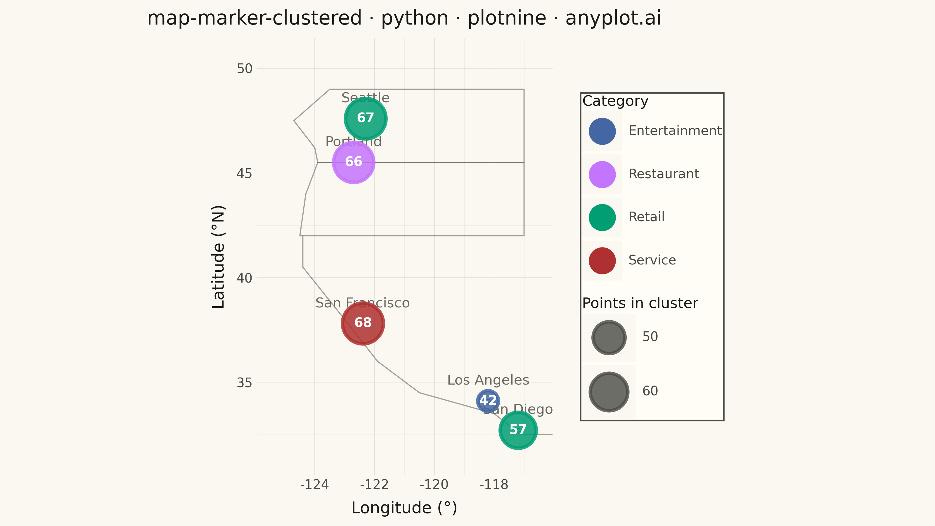
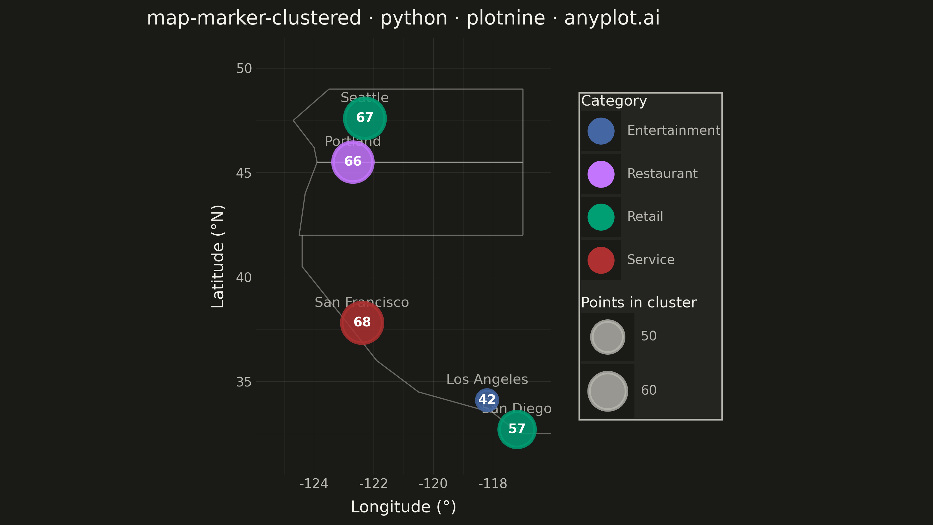
A geographic map that dynamically clusters nearby markers based on the current zoom level. At lower zoom levels, clusters aggregate multiple points into a single marker displaying the count, while zooming in progressively expands clusters to reveal individual markers. This visualization is essential for efficiently displaying large geographic datasets without visual clutter, enabling users to see both the overall distribution and specific locations through interactive exploration.
""" anyplot.ai
map-marker-clustered: Clustered Marker Map
Library: plotnine 0.15.4 | Python 3.13.13
Quality: 86/100 | Updated: 2026-05-23
"""

import os

import numpy as np
import pandas as pd
from plotnine import (
    aes,
    coord_fixed,
    element_blank,
    element_line,
    element_rect,
    element_text,
    geom_path,
    geom_point,
    geom_polygon,
    geom_text,
    ggplot,
    guide_legend,
    guides,
    labs,
    scale_color_manual,
    scale_fill_identity,
    scale_size_continuous,
    theme,
)
from scipy.cluster.hierarchy import fcluster, linkage
from scipy.spatial import ConvexHull


# Theme tokens
THEME = os.getenv("ANYPLOT_THEME", "light")
PAGE_BG = "#FAF8F1" if THEME == "light" else "#1A1A17"
ELEVATED_BG = "#FFFDF6" if THEME == "light" else "#242420"
INK = "#1A1A17" if THEME == "light" else "#F0EFE8"
INK_SOFT = "#4A4A44" if THEME == "light" else "#B8B7B0"
INK_MUTED = "#6B6A63" if THEME == "light" else "#A8A79F"

# Imprint palette — first series is always #009E73
CATEGORY_COLORS = {"Retail": "#009E73", "Restaurant": "#C475FD", "Service": "#AE3030", "Entertainment": "#4467A3"}

# Data: US West Coast retail store locations
np.random.seed(42)

city_centers = {
    "Seattle": (47.6, -122.3),
    "Portland": (45.5, -122.7),
    "San Francisco": (37.8, -122.4),
    "Los Angeles": (34.1, -118.2),
    "San Diego": (32.7, -117.2),
}

# Per-city weighted categories ensure each cluster has a visually distinct dominant color
category_types = ["Retail", "Restaurant", "Service", "Entertainment"]
city_weights = {
    "Seattle": [0.70, 0.10, 0.10, 0.10],  # Retail  → #009E73
    "Portland": [0.10, 0.70, 0.10, 0.10],  # Restaurant → #C475FD
    "San Francisco": [0.10, 0.10, 0.70, 0.10],  # Service → #AE3030
    "Los Angeles": [0.10, 0.10, 0.10, 0.70],  # Entertainment → #4467A3
    "San Diego": [0.70, 0.10, 0.10, 0.10],  # Retail → #009E73 (far from Seattle)
}

n_points = 300
lats, lons, cats = [], [], []

for _ in range(n_points):
    city = np.random.choice(list(city_centers.keys()))
    clat, clon = city_centers[city]
    lats.append(clat + np.random.normal(0, 0.04))
    lons.append(clon + np.random.normal(0, 0.04))
    cats.append(np.random.choice(category_types, p=city_weights[city]))

df = pd.DataFrame({"lat": lats, "lon": lons, "category": cats})

# Hierarchical clustering — force exactly 5 clusters (one per city)
Z = linkage(df[["lat", "lon"]].values, method="ward")
df["cluster"] = fcluster(Z, t=5, criterion="maxclust")

cluster_markers = (
    df.groupby("cluster")
    .agg(
        lat=("lat", "mean"),
        lon=("lon", "mean"),
        count=("cluster", "size"),
        category=("category", lambda x: x.mode().iloc[0]),
    )
    .reset_index()
)
cluster_markers["label"] = cluster_markers["count"].astype(str)

# Convex hull polygons showing each cluster's geographic extent
hull_rows = []
for cluster_id in sorted(df["cluster"].unique()):
    pts = df[df["cluster"] == cluster_id][["lon", "lat"]].values
    if len(pts) >= 3:
        try:
            hull = ConvexHull(pts)
            verts = pts[hull.vertices]
            verts = np.vstack([verts, verts[0]])
            cat = cluster_markers.loc[cluster_markers["cluster"] == cluster_id, "category"].iloc[0]
            for lon_v, lat_v in verts:
                hull_rows.append({"lon": lon_v, "lat": lat_v, "cluster": cluster_id, "category": cat})
        except Exception:
            pass

hull_df = pd.DataFrame(hull_rows)
hull_df["fill_color"] = hull_df["category"].map(CATEGORY_COLORS)

# Simplified West Coast state outlines for geographic context
state_boundaries = pd.concat(
    [
        pd.DataFrame(
            {
                "lat": [45.5, 49.0, 49.0, 47.5, 46.2, 45.5, 45.5],
                "lon": [-117.0, -117.0, -123.5, -124.7, -124.0, -123.9, -117.0],
                "state": "WA",
            }
        ),
        pd.DataFrame(
            {
                "lat": [42.0, 45.5, 45.5, 44.0, 42.0, 42.0],
                "lon": [-117.0, -117.0, -123.9, -124.3, -124.5, -117.0],
                "state": "OR",
            }
        ),
        pd.DataFrame(
            {
                "lat": [42.0, 40.5, 38.0, 36.0, 34.5, 33.5, 32.5, 32.5, 42.0],
                "lon": [-124.4, -124.4, -123.0, -121.9, -120.5, -118.0, -117.1, -114.6, -114.6],
                "state": "CA",
            }
        ),
    ],
    ignore_index=True,
)

# City reference labels for geographic orientation
city_label_df = pd.DataFrame(
    [{"lat": lat + 0.65, "lon": lon, "name": city} for city, (lat, lon) in city_centers.items()]
)

# Plot
plot = (
    ggplot(cluster_markers, aes(x="lon", y="lat"))
    + geom_polygon(
        data=hull_df,
        mapping=aes(x="lon", y="lat", group="cluster", fill="fill_color"),
        alpha=0.13,
        color=INK_SOFT,
        size=0.25,
    )
    + geom_path(
        data=state_boundaries, mapping=aes(x="lon", y="lat", group="state"), color=INK_SOFT, size=0.4, alpha=0.5
    )
    + geom_text(data=city_label_df, mapping=aes(x="lon", y="lat", label="name"), color=INK_MUTED, size=8.5, va="bottom")
    + geom_point(aes(size="count", color="category"), alpha=0.85, stroke=1.2)
    + geom_text(aes(label="label"), size=8, color="white", fontweight="bold")
    + scale_color_manual(values=CATEGORY_COLORS, name="Category")
    + scale_fill_identity()
    + scale_size_continuous(range=(6, 13), name="Points in cluster")
    + coord_fixed(ratio=0.7, xlim=(-125.5, -116.5), ylim=(31.5, 50.5))
    + labs(title="map-marker-clustered · python · plotnine · anyplot.ai", x="Longitude (°)", y="Latitude (°N)")
    + theme(
        figure_size=(8, 4.5),
        plot_background=element_rect(fill=PAGE_BG, color=PAGE_BG),
        panel_background=element_rect(fill=PAGE_BG),
        panel_grid_major=element_line(color=INK, size=0.3, alpha=0.10),
        panel_grid_minor=element_line(color=INK, size=0.2, alpha=0.05),
        panel_border=element_blank(),
        axis_title=element_text(color=INK, size=10),
        axis_text=element_text(color=INK_SOFT, size=8),
        axis_line=element_blank(),
        axis_ticks=element_blank(),
        plot_title=element_text(color=INK, size=12),
        legend_background=element_rect(fill=ELEVATED_BG, color=INK_SOFT),
        legend_text=element_text(color=INK_SOFT, size=8),
        legend_title=element_text(color=INK, size=9),
        legend_position="right",
        legend_box="vertical",
    )
    + guides(
        color=guide_legend(override_aes={"size": 7, "alpha": 1}),
        size=guide_legend(override_aes={"color": INK_SOFT, "alpha": 0.8}),
    )
)

plot.save(f"plot-{THEME}.png", dpi=400, width=8, height=4.5, units="in", verbose=False)
Runnable source as JSON, for any HTTP client: https://api.anyplot.ai/specs/map-marker-clustered/plotnine/code. Any spec id and library id listed in llms-full.txt fit the same URL shape; every URL below is complete and callable.
{
  "spec_id": "map-marker-clustered",
  "language": "python",
  "library": "plotnine",
  "page": "https://anyplot.ai/map-marker-clustered/python/plotnine",
  "hub": "https://anyplot.ai/map-marker-clustered",
  "code_json": "https://api.anyplot.ai/specs/map-marker-clustered/plotnine/code",
  "spec_json": "https://api.anyplot.ai/specs/map-marker-clustered",
  "render_light_png": "https://storage.googleapis.com/anyplot-images/plots/map-marker-clustered/python/plotnine/plot-light.png",
  "render_dark_png": "https://storage.googleapis.com/anyplot-images/plots/map-marker-clustered/python/plotnine/plot-dark.png",
  "quality_score": 86.0,
  "license": "MIT",
  "guide": "https://anyplot.ai/llms.txt"
}
Part of Clustered Marker Map on anyplot.ai.