The same plot in 14 other libraries — Python: Altair, Bokeh, lets-plot, Matplotlib, Plotly, plotnine, Seaborn; R: ggplot2; Julia: Makie.jl; JavaScript: Chart.js, D3.js, Apache ECharts, Highcharts, MUI X Charts. Compare all 15 side by side: Clustered Marker Map in Python, R, Julia and JavaScript.
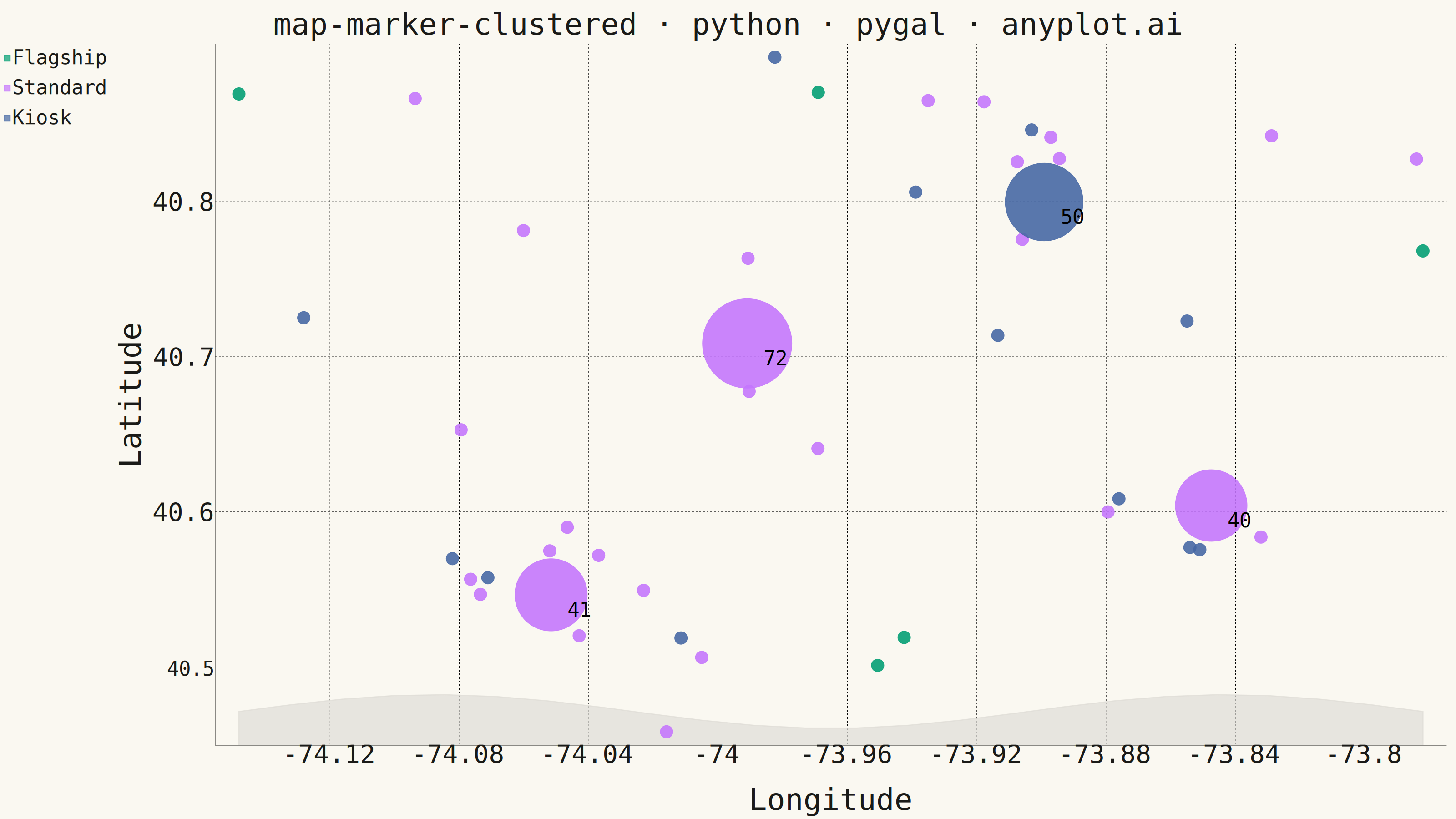
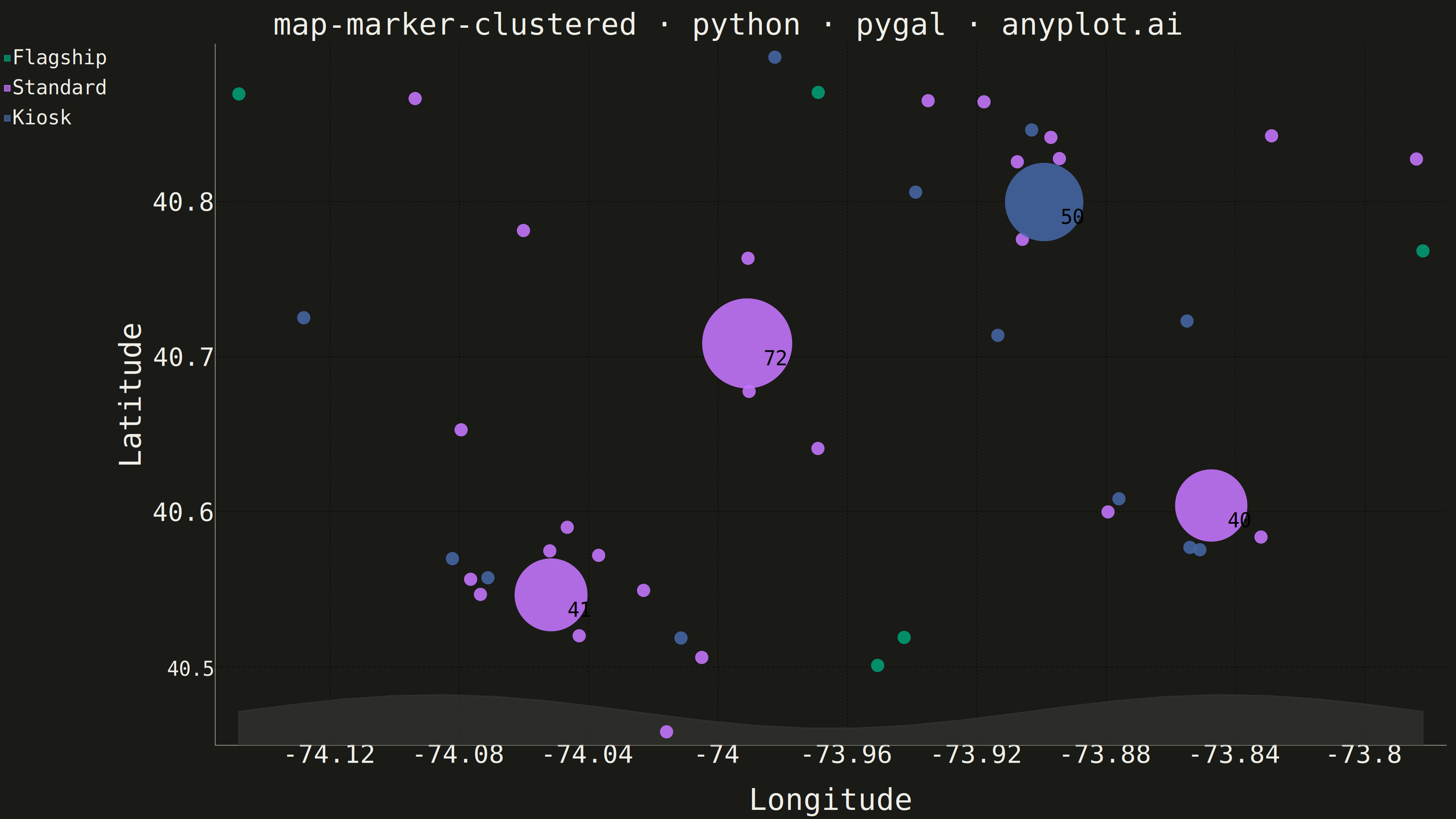
A geographic map that dynamically clusters nearby markers based on the current zoom level. At lower zoom levels, clusters aggregate multiple points into a single marker displaying the count, while zooming in progressively expands clusters to reveal individual markers. This visualization is essential for efficiently displaying large geographic datasets without visual clutter, enabling users to see both the overall distribution and specific locations through interactive exploration.
""" anyplot.ai
map-marker-clustered: Clustered Marker Map
Library: pygal 3.1.3 | Python 3.13.15
Quality: 84/100 | Created: 2026-08-24
"""

import os
from collections import Counter

import numpy as np
import pygal
from pygal.style import Style
from sklearn.cluster import DBSCAN


# Theme tokens (see prompts/default-style-guide.md "Theme-adaptive Chrome")
THEME = os.getenv("ANYPLOT_THEME", "light")
PAGE_BG = "#FAF8F1" if THEME == "light" else "#1A1A17"
INK = "#1A1A17" if THEME == "light" else "#F0EFE8"
INK_MUTED = "#6B6A63" if THEME == "light" else "#A8A79F"

# Imprint categorical palette — first series is always the brand green
IMPRINT_PALETTE = ("#009E73", "#C475FD", "#4467A3", "#BD8233", "#AE3030", "#2ABCCD", "#954477", "#99B314")

# Data — synthetic coffee-shop chain locations across a metro area
np.random.seed(42)

CATEGORIES = ["Flagship", "Standard", "Kiosk"]
CATEGORY_WEIGHTS = [0.10, 0.55, 0.35]

# (center_lat, center_lon, point_count, spread_degrees)
hubs = [
    (40.71, -73.99, 70, 0.010),  # downtown core
    (40.80, -73.90, 55, 0.012),  # riverside district
    (40.60, -73.85, 45, 0.012),  # uptown district
    (40.55, -74.05, 50, 0.013),  # harbor district
]

lats, lons, cats = [], [], []
for center_lat, center_lon, point_count, spread in hubs:
    lats.extend(np.random.normal(center_lat, spread, point_count))
    lons.extend(np.random.normal(center_lon, spread, point_count))
    cats.extend(np.random.choice(CATEGORIES, point_count, p=CATEGORY_WEIGHTS))

n_outlying = 25
lats.extend(np.random.uniform(40.45, 40.90, n_outlying))
lons.extend(np.random.uniform(-74.15, -73.75, n_outlying))
cats.extend(np.random.choice(CATEGORIES, n_outlying, p=CATEGORY_WEIGHTS))

lats = np.array(lats)
lons = np.array(lons)
cats = np.array(cats)

# Minimal geographic reference layer: a soft coastline band along the
# southern edge, shaded on the water side, so the plot reads as a map
# rather than a plain scatter even without a tile basemap. Built purely
# from theme tokens (no new brand colors).
lat_min, lat_max = float(lats.min()), float(lats.max())
lon_min, lon_max = float(lons.min()), float(lons.max())
lat_span = lat_max - lat_min
WATER_FILL = "#{:02X}{:02X}{:02X}".format(
    *(round(int(PAGE_BG[i : i + 2], 16) * 0.88 + int(INK[i : i + 2], 16) * 0.12) for i in (1, 3, 5))
)
coastline_x = np.linspace(lon_min, lon_max, 24)
coastline_y = lat_min + lat_span * (0.03 + 0.025 * np.sin(np.linspace(0, 3 * np.pi, 24)))
water_band = list(zip(coastline_x.tolist(), coastline_y.tolist(), strict=True))

# Cluster nearby stores the way a map would collapse them at a fixed zoom
# level; isolated stores (label -1) stay as individual markers.
cluster_labels = DBSCAN(eps=0.012, min_samples=8).fit_predict(np.column_stack([lats, lons]))

INDIVIDUAL_RADIUS = 14
CLUSTER_RADIUS_BASE = 22
CLUSTER_RADIUS_SCALE = 9

series_points = {category: [] for category in CATEGORIES}
for label in sorted(set(cluster_labels)):
    members = cluster_labels == label
    if label == -1:
        for lat, lon, category in zip(lats[members], lons[members], cats[members], strict=True):
            series_points[category].append(
                {"value": (lon, lat), "node": {"r": INDIVIDUAL_RADIUS}, "tooltip": f"{category} store"}
            )
    else:
        count = int(members.sum())
        dominant_category = Counter(cats[members]).most_common(1)[0][0]
        centroid_lon = float(lons[members].mean())
        centroid_lat = float(lats[members].mean())
        radius = CLUSTER_RADIUS_BASE + CLUSTER_RADIUS_SCALE * count**0.5
        series_points[dominant_category].append(
            {
                "value": (centroid_lon, centroid_lat),
                "node": {"r": round(radius, 1)},
                "label": str(count),
                "tooltip": f"{count} stores clustered here ({dominant_category} dominant)",
            }
        )

# Style — title kept compact because the mandated anyplot title is ~67 chars long
TITLE = "map-marker-clustered · python · pygal · anyplot.ai"
title_ratio = 67 / len(TITLE) if len(TITLE) > 67 else 1.0
title_font_size = max(44, round(66 * title_ratio))

custom_style = Style(
    background=PAGE_BG,
    plot_background=PAGE_BG,
    foreground=INK,
    foreground_strong=INK,
    foreground_subtle=INK_MUTED,
    colors=(WATER_FILL, *IMPRINT_PALETTE[: len(CATEGORIES)]),
    title_font_size=title_font_size,
    label_font_size=56,
    major_label_font_size=44,
    legend_font_size=44,
    value_font_size=36,
    value_label_font_size=44,
    dot_opacity=0.88,
    stroke_width=2.5,
)

# Plot — an XY scatter stands in for the map surface, with a coastline
# fill layer beneath it for geographic context; circle size encodes
# cluster size and the printed number is the grouped-point count.
chart = pygal.XY(
    style=custom_style,
    width=3200,
    height=1800,
    title=TITLE,
    x_title="Longitude",
    y_title="Latitude",
    stroke=False,
    show_dots=True,
    print_labels=True,
    print_values=False,
    show_x_guides=True,
    show_y_guides=True,
    show_legend=True,
)

# Water-side fill beneath the coastline curve; title=None keeps it out
# of the category legend since it isn't a data series.
chart.add(None, water_band, stroke=True, fill=True, show_dots=False, stroke_style={"width": 2})

for category in CATEGORIES:
    chart.add(category, series_points[category])

# Save
chart.render_to_png(f"plot-{THEME}.png")
with open(f"plot-{THEME}.html", "wb") as f:
    f.write(chart.render())
Runnable source as JSON, for any HTTP client: https://api.anyplot.ai/specs/map-marker-clustered/pygal/code. Any spec id and library id listed in llms-full.txt fit the same URL shape; every URL below is complete and callable.
{
  "spec_id": "map-marker-clustered",
  "language": "python",
  "library": "pygal",
  "page": "https://anyplot.ai/map-marker-clustered/python/pygal",
  "hub": "https://anyplot.ai/map-marker-clustered",
  "code_json": "https://api.anyplot.ai/specs/map-marker-clustered/pygal/code",
  "spec_json": "https://api.anyplot.ai/specs/map-marker-clustered",
  "render_light_png": "https://storage.googleapis.com/anyplot-images/plots/map-marker-clustered/python/pygal/plot-light.png",
  "render_dark_png": "https://storage.googleapis.com/anyplot-images/plots/map-marker-clustered/python/pygal/plot-dark.png",
  "interactive_light_html": "https://storage.googleapis.com/anyplot-images/plots/map-marker-clustered/python/pygal/plot-light.html",
  "interactive_dark_html": "https://storage.googleapis.com/anyplot-images/plots/map-marker-clustered/python/pygal/plot-dark.html",
  "quality_score": 84.0,
  "license": "MIT",
  "guide": "https://anyplot.ai/llms.txt"
}
Part of Clustered Marker Map on anyplot.ai.