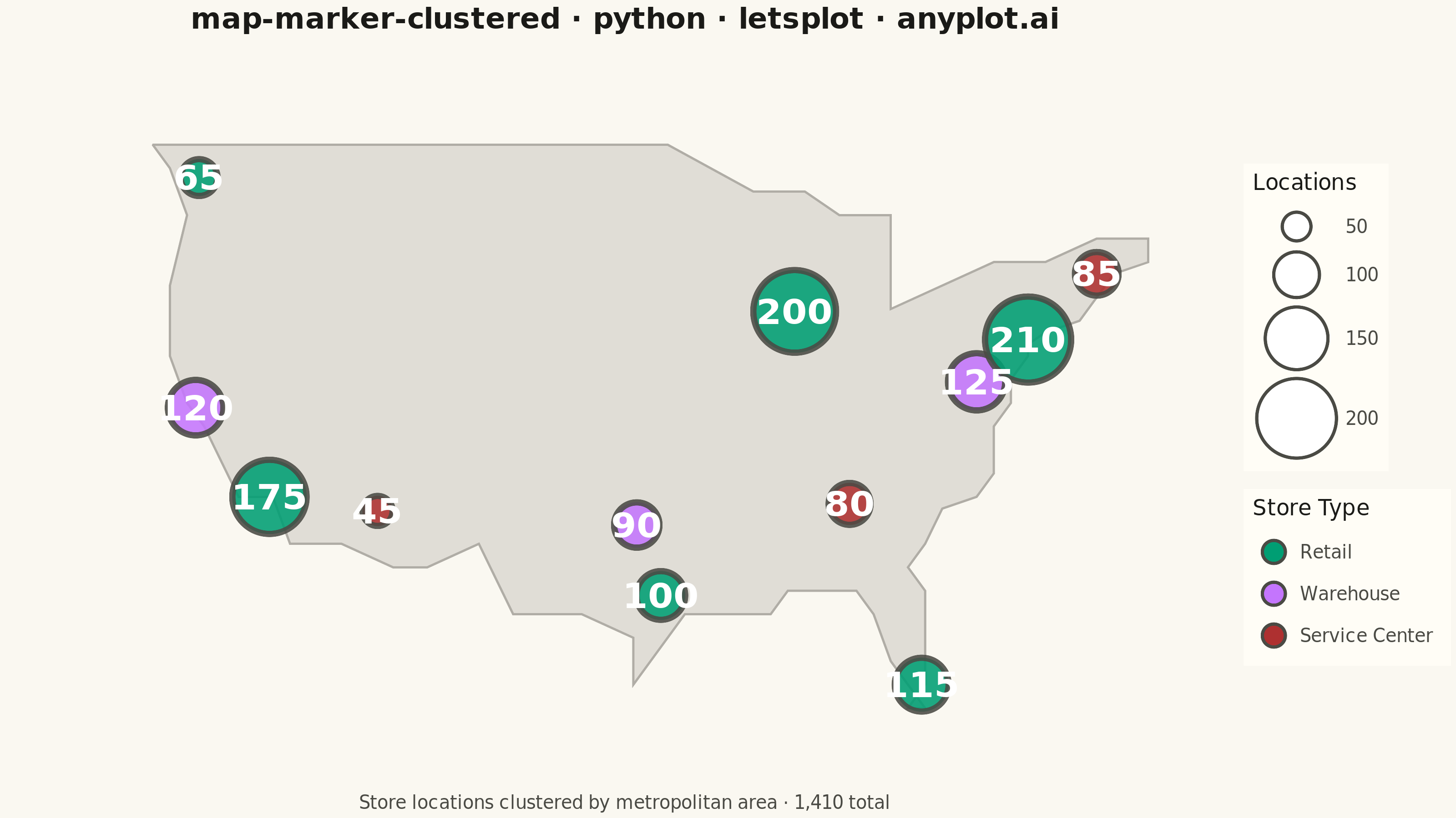
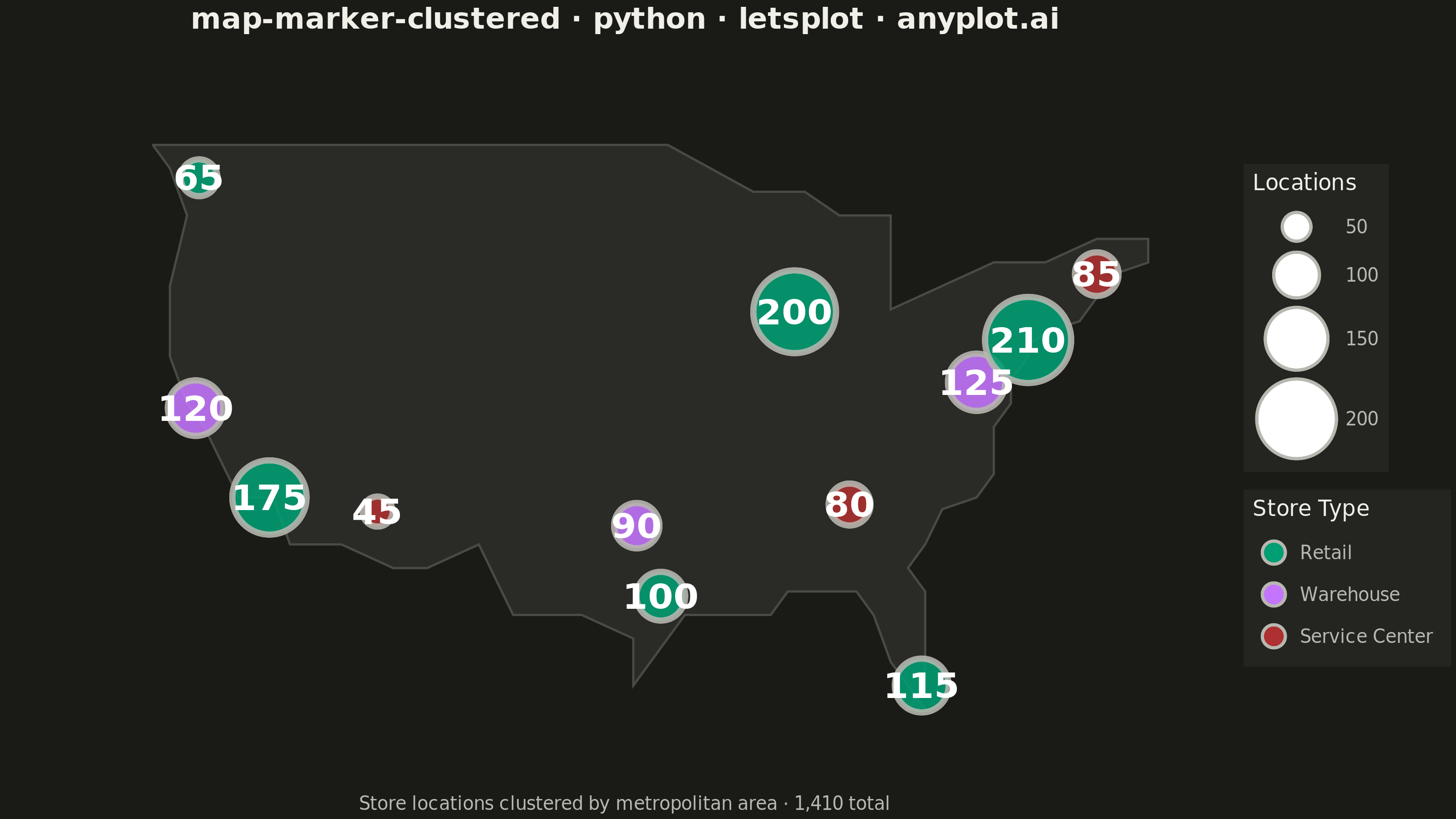
A geographic map that dynamically clusters nearby markers based on the current zoom level. At lower zoom levels, clusters aggregate multiple points into a single marker displaying the count, while zooming in progressively expands clusters to reveal individual markers. This visualization is essential for efficiently displaying large geographic datasets without visual clutter, enabling users to see both the overall distribution and specific locations through interactive exploration.
""" anyplot.ai
map-marker-clustered: Clustered Marker Map
Library: letsplot 4.10.1 | Python 3.13.13
Quality: 86/100 | Updated: 2026-05-23
"""

import os

import pandas as pd
from lets_plot import (
    LetsPlot,
    aes,
    element_rect,
    element_text,
    geom_point,
    geom_polygon,
    geom_text,
    ggplot,
    ggsave,
    ggsize,
    labs,
    layer_tooltips,
    scale_fill_manual,
    scale_size,
    theme,
    theme_void,
    xlim,
    ylim,
)


LetsPlot.setup_html()

THEME = os.getenv("ANYPLOT_THEME", "light")
PAGE_BG = "#FAF8F1" if THEME == "light" else "#1A1A17"
ELEVATED_BG = "#FFFDF6" if THEME == "light" else "#242420"
INK = "#1A1A17" if THEME == "light" else "#F0EFE8"
INK_SOFT = "#4A4A44" if THEME == "light" else "#B8B7B0"

# Cluster data: pre-aggregated store locations across US metropolitan areas
# New England nudged north-east to reduce visual overlap with NYC cluster
df_clusters = pd.DataFrame(
    {
        "region": [
            "Los Angeles",
            "San Francisco",
            "Pacific Northwest",
            "Desert Southwest",
            "Chicago",
            "Dallas",
            "Houston",
            "Southeast",
            "South Florida",
            "Washington DC",
            "New York City",
            "New England",
        ],
        "lon": [-118.2, -122.5, -122.3, -111.9, -87.6, -96.8, -95.4, -84.4, -80.2, -77.0, -74.0, -70.0],
        "lat": [34.0, 37.8, 47.6, 33.4, 41.9, 32.8, 29.8, 33.7, 26.0, 38.9, 40.7, 43.5],
        "count": [175, 120, 65, 45, 200, 90, 100, 80, 115, 125, 210, 85],
        "category": [
            "Retail",
            "Warehouse",
            "Retail",
            "Service Center",
            "Retail",
            "Warehouse",
            "Retail",
            "Service Center",
            "Retail",
            "Warehouse",
            "Retail",
            "Service Center",
        ],
    }
)

# Imprint palette — canonical order for categorical data
colors = {"Retail": "#009E73", "Warehouse": "#C475FD", "Service Center": "#AE3030"}

# Higher-fidelity US continental boundary polygon (66 vertices vs prior 44)
us_boundary = [
    # Canadian border west to east
    (-125, 49),
    (-120, 49),
    (-115, 49),
    (-110, 49),
    (-105, 49),
    (-100, 49),
    (-95, 49),
    (-90, 47),
    (-87, 47),
    # Great Lakes south shoreline
    (-85, 46),
    (-82, 46),
    (-82, 42),
    (-79, 43),
    (-76, 44),
    (-73, 44),
    # Maine and New England coast
    (-70, 45),
    (-67, 45),
    (-67, 44),
    (-69, 43.5),
    (-70, 42.5),
    (-71, 41.5),
    (-73, 41),
    # Mid-Atlantic
    (-74, 40.5),
    (-74, 40),
    (-75, 39),
    (-75, 38),
    # Southeast Atlantic coast
    (-76, 37),
    (-76, 36),
    (-76, 35),
    (-77, 34),
    (-79, 33.5),
    (-80, 32),
    (-81, 31),
    (-80, 30),
    (-80, 28),
    # Florida peninsula
    (-80, 26),
    (-81, 25),
    (-80, 25),
    # Florida west coast and Gulf of Mexico
    (-82, 27),
    (-83, 29),
    (-84, 30),
    (-86, 30),
    (-88, 30),
    (-89, 29),
    (-90, 29),
    (-91, 29),
    (-94, 29),
    # Texas Gulf coast
    (-97, 26),
    (-97, 27),
    (-97, 28),
    (-100, 29),
    (-104, 29),
    # Southwest border
    (-106, 32),
    (-109, 31),
    (-111, 31),
    (-114, 32),
    # Pacific coast
    (-117, 32),
    (-118, 34),
    (-120, 34),
    (-122, 37),
    (-123, 38),
    (-124, 40),
    (-124, 43),
    (-123, 46),
    (-124, 48),
    (-125, 49),
]
df_us = pd.DataFrame(us_boundary, columns=["x", "y"])
df_us["group"] = 0

map_fill = "#E0DDD6" if THEME == "light" else "#2A2A27"
map_border = "#B0ADA6" if THEME == "light" else "#4A4A44"

plot = (
    ggplot()
    + geom_polygon(data=df_us, mapping=aes(x="x", y="y", group="group"), fill=map_fill, color=map_border, size=0.5)
    + geom_point(
        data=df_clusters,
        mapping=aes(x="lon", y="lat", size="count", fill="category"),
        color=INK_SOFT,
        alpha=0.88,
        shape=21,
        stroke=1.5,
        tooltips=layer_tooltips().title("@region").line("@count locations").line("Type|@category"),
    )
    + geom_text(
        data=df_clusters, mapping=aes(x="lon", y="lat", label="count"), color="#FFFFFF", size=10, fontface="bold"
    )
    + scale_fill_manual(values=colors, name="Store Type")
    + scale_size(range=[6, 20], name="Locations", breaks=[50, 100, 150, 200])
    + labs(
        title="map-marker-clustered · python · letsplot · anyplot.ai",
        caption="Store locations clustered by metropolitan area · 1,410 total",
    )
    + theme_void()
    + theme(
        plot_title=element_text(size=16, hjust=0.5, face="bold", color=INK),
        plot_caption=element_text(size=10, hjust=0.5, color=INK_SOFT),
        legend_title=element_text(size=12, color=INK),
        legend_text=element_text(size=10, color=INK_SOFT),
        legend_position="right",
        plot_background=element_rect(fill=PAGE_BG, color=PAGE_BG),
        legend_background=element_rect(fill=ELEVATED_BG, color=INK_SOFT),
    )
    + ggsize(800, 450)
    + xlim(-130, -65)
    + ylim(23, 52)
)

ggsave(plot, f"plot-{THEME}.png", scale=4, path=".")
ggsave(plot, f"plot-{THEME}.html", path=".")
Runnable source as JSON, for any HTTP client: https://api.anyplot.ai/specs/map-marker-clustered/letsplot/code. Any spec id and library id listed in llms-full.txt fit the same URL shape; every URL below is complete and callable.
{
  "spec_id": "map-marker-clustered",
  "language": "python",
  "library": "letsplot",
  "page": "https://anyplot.ai/map-marker-clustered/python/letsplot",
  "hub": "https://anyplot.ai/map-marker-clustered",
  "code_json": "https://api.anyplot.ai/specs/map-marker-clustered/letsplot/code",
  "spec_json": "https://api.anyplot.ai/specs/map-marker-clustered",
  "render_light_png": "https://storage.googleapis.com/anyplot-images/plots/map-marker-clustered/python/letsplot/plot-light.png",
  "render_dark_png": "https://storage.googleapis.com/anyplot-images/plots/map-marker-clustered/python/letsplot/plot-dark.png",
  "interactive_light_html": "https://storage.googleapis.com/anyplot-images/plots/map-marker-clustered/python/letsplot/plot-light.html",
  "interactive_dark_html": "https://storage.googleapis.com/anyplot-images/plots/map-marker-clustered/python/letsplot/plot-dark.html",
  "quality_score": 86.0,
  "license": "MIT",
  "guide": "https://anyplot.ai/llms.txt"
}
Part of Clustered Marker Map on anyplot.ai.