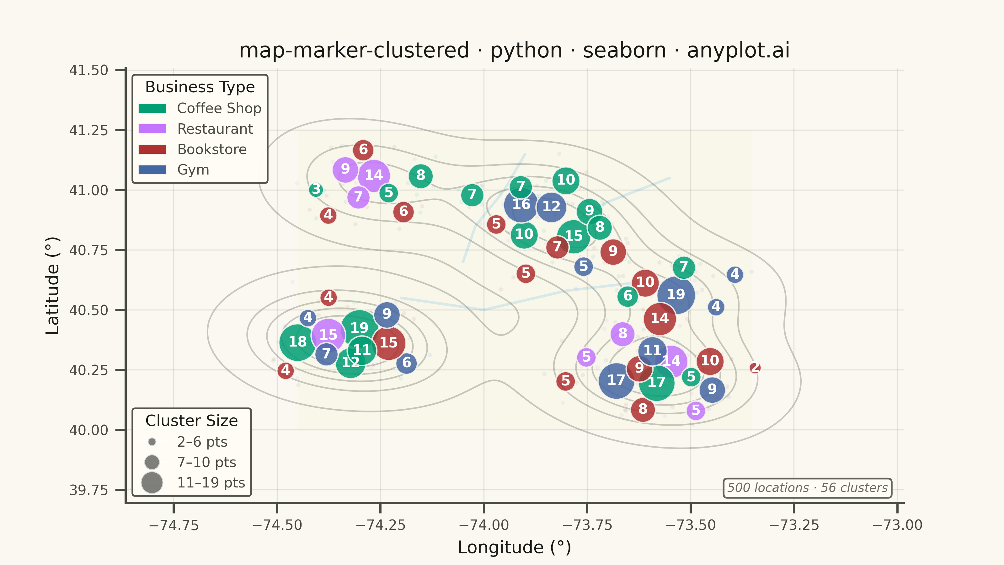
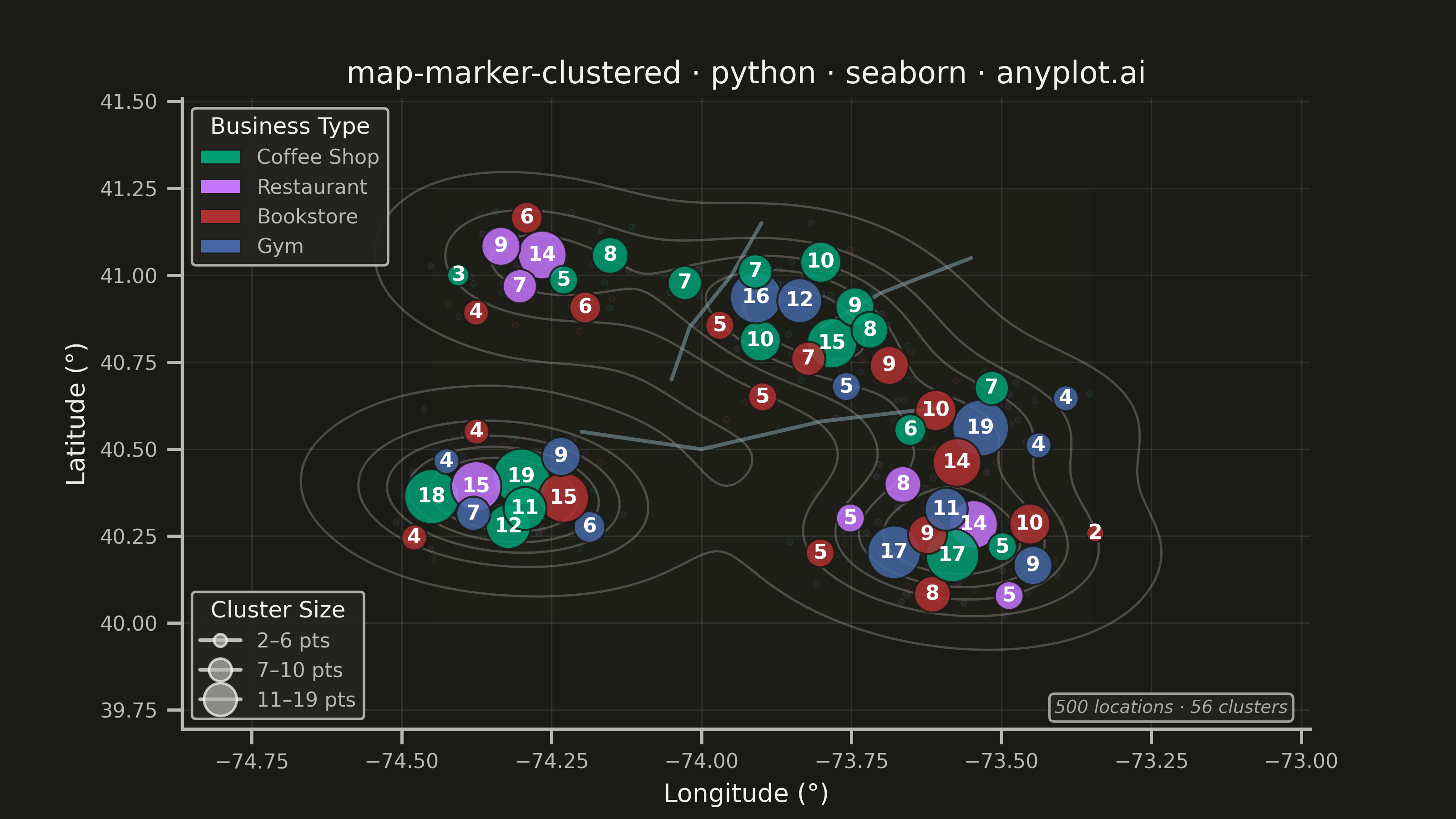
A geographic map that dynamically clusters nearby markers based on the current zoom level. At lower zoom levels, clusters aggregate multiple points into a single marker displaying the count, while zooming in progressively expands clusters to reveal individual markers. This visualization is essential for efficiently displaying large geographic datasets without visual clutter, enabling users to see both the overall distribution and specific locations through interactive exploration.
""" anyplot.ai
map-marker-clustered: Clustered Marker Map
Library: seaborn 0.13.2 | Python 3.13.13
Quality: 89/100 | Updated: 2026-05-23
"""

import os

import matplotlib.patches as mpatches
import matplotlib.pyplot as plt
import numpy as np
import pandas as pd
import seaborn as sns
from matplotlib.lines import Line2D
from sklearn.cluster import AgglomerativeClustering


# Theme tokens
THEME = os.getenv("ANYPLOT_THEME", "light")
PAGE_BG = "#FAF8F1" if THEME == "light" else "#1A1A17"
ELEVATED_BG = "#FFFDF6" if THEME == "light" else "#242420"
INK = "#1A1A17" if THEME == "light" else "#F0EFE8"
INK_SOFT = "#4A4A44" if THEME == "light" else "#B8B7B0"
INK_MUTED = "#6B6A63" if THEME == "light" else "#A8A79F"

# Imprint palette — canonical order, 4 categories
IMPRINT = ["#009E73", "#C475FD", "#AE3030", "#4467A3"]
category_names = ["Coffee Shop", "Restaurant", "Bookstore", "Gym"]
category_palette = dict(zip(category_names, IMPRINT, strict=True))

# Data — business locations across NYC region
np.random.seed(42)
n_points = 500

n_neighborhoods = 8
neighborhood_centers = np.random.uniform(-0.5, 0.5, (n_neighborhoods, 2))
points_per_neighborhood = n_points // n_neighborhoods

lats, lons, categories = [], [], []
for i, center in enumerate(neighborhood_centers):
    n_pts = points_per_neighborhood + (n_points % n_neighborhoods if i == 0 else 0)
    lat = np.random.normal(center[0], 0.08, n_pts) + 40.7
    lon = np.random.normal(center[1], 0.08, n_pts) - 74.0
    lats.extend(lat)
    lons.extend(lon)
    categories.extend(np.random.choice(category_names, n_pts))

df = pd.DataFrame({"lat": lats, "lon": lons, "category": categories})

# Apply hierarchical clustering to group nearby markers
coords = df[["lat", "lon"]].values
clustering = AgglomerativeClustering(n_clusters=None, distance_threshold=0.18, linkage="ward")
df["cluster"] = clustering.fit_predict(coords)

# Cluster centers, sizes and dominant category
cluster_stats = (
    df.groupby("cluster")
    .agg(
        lat_center=("lat", "mean"),
        lon_center=("lon", "mean"),
        count=("lat", "size"),
        dominant_category=("category", lambda x: x.mode().iloc[0]),
    )
    .reset_index()
)

# Compute actual cluster size thresholds for accurate legend labels
count_min = int(cluster_stats["count"].min())
count_p33 = int(cluster_stats["count"].quantile(0.33))
count_p66 = int(cluster_stats["count"].quantile(0.66))
count_max = int(cluster_stats["count"].max())

# Set seaborn theme with theme-adaptive chrome
sns.set_theme(
    style="ticks",
    rc={
        "figure.facecolor": PAGE_BG,
        "axes.facecolor": PAGE_BG,
        "axes.edgecolor": INK_SOFT,
        "axes.labelcolor": INK,
        "text.color": INK,
        "xtick.color": INK_SOFT,
        "ytick.color": INK_SOFT,
        "grid.color": INK,
        "grid.alpha": 0.10,
        "legend.facecolor": ELEVATED_BG,
        "legend.edgecolor": INK_SOFT,
    },
)

# Plot
fig, ax = plt.subplots(figsize=(8, 4.5), dpi=400, facecolor=PAGE_BG)
ax.set_facecolor(PAGE_BG)

# Geographic context — stylized NYC region water boundaries
hudson_river = [(-74.05, 40.70), (-74.02, 40.85), (-73.95, 41.00), (-73.90, 41.15)]
li_sound = [(-73.80, 40.85), (-73.70, 40.95), (-73.55, 41.05)]
coast = [(-74.20, 40.55), (-74.00, 40.50), (-73.80, 40.58), (-73.60, 40.62)]

for segment in [hudson_river, li_sound, coast]:
    xs, ys = zip(*segment, strict=True)
    ax.plot(xs, ys, color="#a8d4e6", linewidth=1.5, alpha=0.4, zorder=0, solid_capstyle="round")

land_fill = "#f5f5dc" if THEME == "light" else "#2a2a20"
land_patch = mpatches.Polygon(
    [(-74.45, 40.0), (-74.45, 41.25), (-73.35, 41.25), (-73.35, 40.0)],
    facecolor=land_fill,
    edgecolor="none",
    alpha=0.3,
    zorder=-1,
)
ax.add_patch(land_patch)

# KDE density contours — seaborn-distinctive statistical overlay showing point density
sns.kdeplot(data=df, x="lon", y="lat", levels=6, color=INK_MUTED, alpha=0.35, linewidths=0.9, ax=ax, zorder=1)

# Background layer — individual points at minimal alpha
sns.scatterplot(
    data=df, x="lon", y="lat", hue="category", palette=category_palette, s=6, alpha=0.08, ax=ax, legend=False
)

# Foreground layer — cluster markers sized by count
sns.scatterplot(
    data=cluster_stats,
    x="lon_center",
    y="lat_center",
    size="count",
    hue="dominant_category",
    palette=category_palette,
    sizes=(50, 500),
    alpha=0.85,
    edgecolor=PAGE_BG,
    linewidth=0.8,
    ax=ax,
    legend=False,
)

# Count labels on clusters
for _, row in cluster_stats.iterrows():
    if row["count"] > 1:
        ax.annotate(
            str(int(row["count"])),
            (row["lon_center"], row["lat_center"]),
            ha="center",
            va="center",
            fontsize=8,
            fontweight="bold",
            color="white",
            zorder=10,
        )

# Category legend
cat_handles = [
    mpatches.Patch(facecolor=category_palette[cat], edgecolor=PAGE_BG, linewidth=0.5, label=cat)
    for cat in category_names
]
cat_legend = ax.legend(
    handles=cat_handles,
    title="Business Type",
    loc="upper left",
    fontsize=8,
    title_fontsize=9,
    framealpha=0.95,
    facecolor=ELEVATED_BG,
    edgecolor=INK_SOFT,
)
cat_legend.get_title().set_color(INK)
for text in cat_legend.get_texts():
    text.set_color(INK_SOFT)

# Size legend — labels derived from actual computed cluster size ranges
small_label = f"{count_min} pt" if count_min == count_p33 else f"{count_min}–{count_p33} pts"
medium_label = f"{count_p33 + 1} pt" if count_p33 + 1 == count_p66 else f"{count_p33 + 1}–{count_p66} pts"
large_label = f"{count_p66 + 1}–{count_max} pts" if count_p66 + 1 < count_max else f"{count_max}+ pts"

size_handles = [
    Line2D([0], [0], marker="o", color="w", markerfacecolor=INK_SOFT, markersize=5, alpha=0.7, label=small_label),
    Line2D([0], [0], marker="o", color="w", markerfacecolor=INK_SOFT, markersize=9, alpha=0.7, label=medium_label),
    Line2D([0], [0], marker="o", color="w", markerfacecolor=INK_SOFT, markersize=13, alpha=0.7, label=large_label),
]
size_legend = ax.legend(
    handles=size_handles,
    title="Cluster Size",
    loc="lower left",
    fontsize=8,
    title_fontsize=9,
    framealpha=0.95,
    facecolor=ELEVATED_BG,
    edgecolor=INK_SOFT,
)
size_legend.get_title().set_color(INK)
for text in size_legend.get_texts():
    text.set_color(INK_SOFT)
ax.add_artist(cat_legend)

# Style
ax.set_xlabel("Longitude (°)", fontsize=10, color=INK)
ax.set_ylabel("Latitude (°)", fontsize=10, color=INK)
ax.set_title("map-marker-clustered · python · seaborn · anyplot.ai", fontsize=12, fontweight="medium", color=INK)
ax.tick_params(axis="both", labelsize=8, colors=INK_SOFT)

sns.despine(ax=ax, left=False, bottom=False)
ax.spines["left"].set_color(INK_SOFT)
ax.spines["bottom"].set_color(INK_SOFT)
ax.grid(True, alpha=0.10, linestyle="-", linewidth=0.6, color=INK)

# Summary annotation (lower right, away from size legend)
ax.text(
    0.98,
    0.02,
    f"{n_points} locations · {len(cluster_stats)} clusters",
    transform=ax.transAxes,
    fontsize=7,
    ha="right",
    va="bottom",
    style="italic",
    color=INK_MUTED,
    bbox={"boxstyle": "round,pad=0.3", "facecolor": ELEVATED_BG, "alpha": 0.85, "edgecolor": INK_SOFT},
)

# Save
plt.savefig(f"plot-{THEME}.png", dpi=400, facecolor=PAGE_BG)
Runnable source as JSON, for any HTTP client: https://api.anyplot.ai/specs/map-marker-clustered/seaborn/code. Any spec id and library id listed in llms-full.txt fit the same URL shape; every URL below is complete and callable.
{
  "spec_id": "map-marker-clustered",
  "language": "python",
  "library": "seaborn",
  "page": "https://anyplot.ai/map-marker-clustered/python/seaborn",
  "hub": "https://anyplot.ai/map-marker-clustered",
  "code_json": "https://api.anyplot.ai/specs/map-marker-clustered/seaborn/code",
  "spec_json": "https://api.anyplot.ai/specs/map-marker-clustered",
  "render_light_png": "https://storage.googleapis.com/anyplot-images/plots/map-marker-clustered/python/seaborn/plot-light.png",
  "render_dark_png": "https://storage.googleapis.com/anyplot-images/plots/map-marker-clustered/python/seaborn/plot-dark.png",
  "quality_score": 89.0,
  "license": "MIT",
  "guide": "https://anyplot.ai/llms.txt"
}
Part of Clustered Marker Map on anyplot.ai.