The same plot in 14 other libraries — Python: Altair, Bokeh, lets-plot, Matplotlib, Plotly, plotnine, Pygal, Seaborn; Julia: Makie.jl; JavaScript: Chart.js, D3.js, Apache ECharts, Highcharts, MUI X Charts. Compare all 15 side by side: Static Transport Network Diagram in Python, R, Julia and JavaScript.
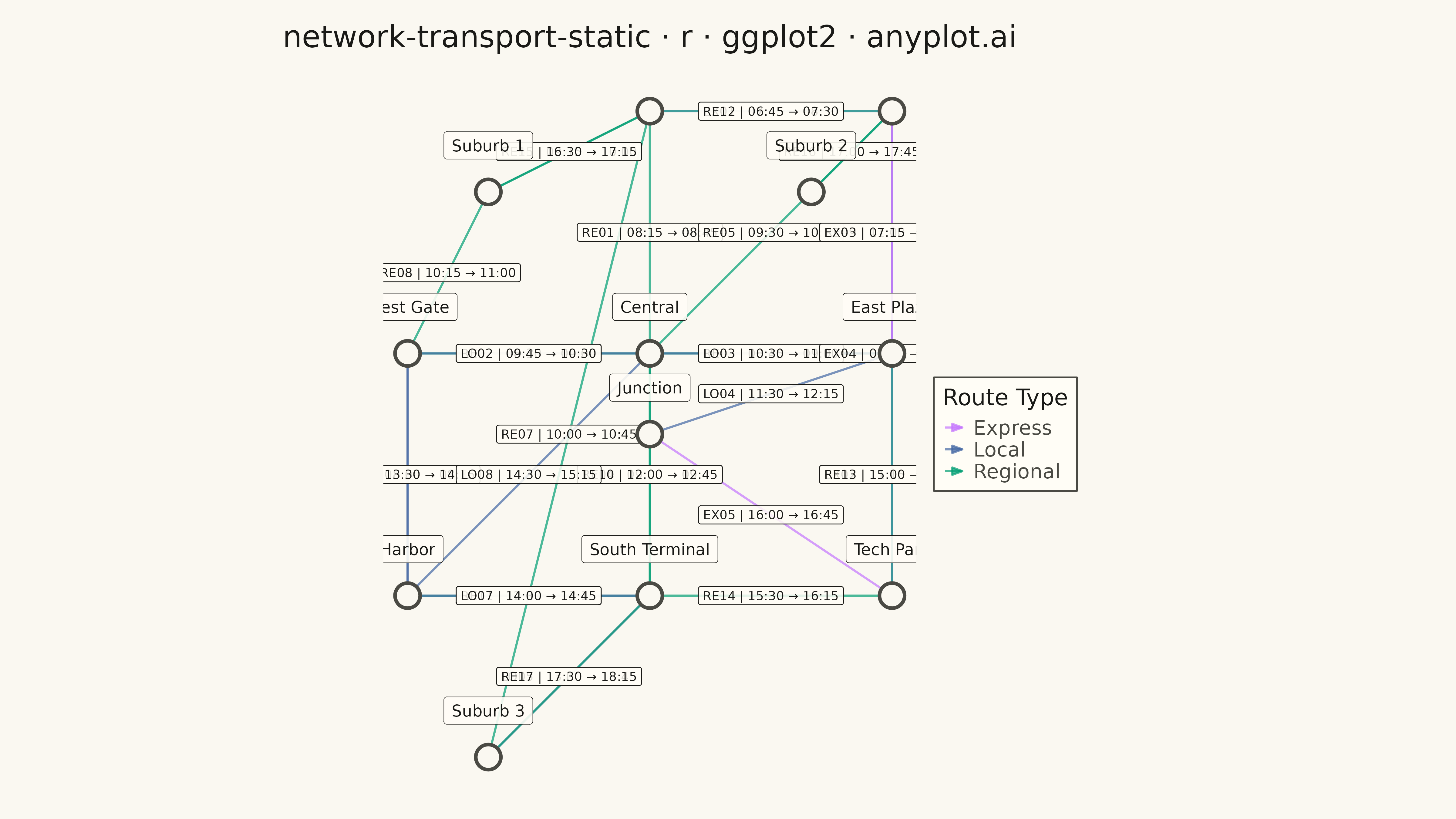
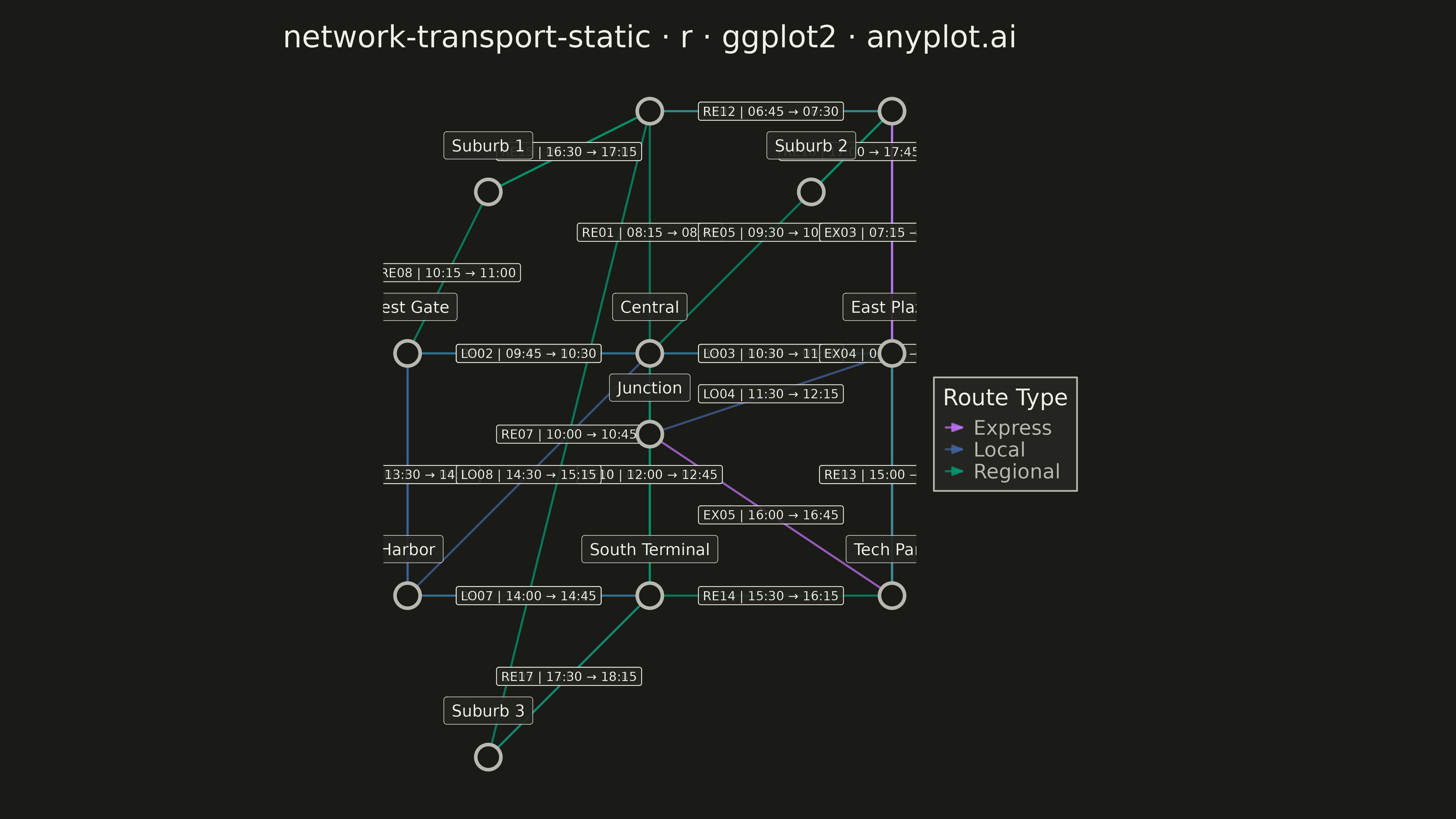
A directed network visualization for transportation systems where stations are displayed as labeled nodes and train/bus routes as directed edges. Edges display departure times, arrival times, and route identifiers. Designed for visualizing timetables, route maps, and connection patterns in rail, bus, or flight networks. This static version focuses on clear, readable presentation without interactive repositioning.
#' anyplot.ai
#' network-transport-static: Static Transport Network Diagram
#' Library: ggplot2 3.5.1 | R 4.4.1
#' Quality: 88/100 | Created: 2026-05-18

library(ggplot2)
library(dplyr)
library(tidyr)
library(ragg)
library(grid)

set.seed(42)

# --- Theme tokens -----------------------------------------------------------
THEME       <- Sys.getenv("ANYPLOT_THEME", "light")
PAGE_BG     <- if (THEME == "light") "#FAF8F1" else "#1A1A17"
ELEVATED_BG <- if (THEME == "light") "#FFFDF6" else "#242420"
INK         <- if (THEME == "light") "#1A1A17" else "#F0EFE8"
INK_SOFT    <- if (THEME == "light") "#4A4A44" else "#B8B7B0"
INK_MUTED   <- if (THEME == "light") "#6B6A63" else "#A8A79F"

IMPRINT   <- c(
  "#009E73",  # 1 — regional (first categorical series)
  "#C475FD",  # 2 — express
  "#4467A3"   # 3 — local
)

# --- Data: Regional rail network with 12 stations and 30 routes ----------------
stations <- data.frame(
  id    = 1:12,
  label = c("Central", "North Hub", "West Gate", "East Plaza", "South Terminal",
            "Airport", "Harbor", "Tech Park", "Suburb 1", "Suburb 2", "Suburb 3", "Junction"),
  x     = c(5, 5, 2, 8, 5, 8, 2, 8, 3, 7, 3, 5),
  y     = c(6, 9, 6, 6, 3, 9, 3, 3, 8, 8, 1, 5),
  stringsAsFactors = FALSE
)

routes <- data.frame(
  source_id = c(1, 1, 1, 1, 1, 2, 2, 2, 3, 3, 3, 4, 4, 4, 4, 5, 5, 5, 6, 6, 6, 7, 7, 7, 8, 8, 8, 9, 10, 11),
  target_id = c(2, 3, 4, 5, 6, 6, 9, 11, 7, 1, 9, 1, 6, 8, 12, 1, 7, 11, 2, 4, 8, 3, 5, 1, 4, 5, 12, 2, 6, 5),
  route_id = c("RE01", "RE02", "RE03", "RE04", "RE05", "EX01", "RE06", "RE07", "LO01", "LO02", "RE08", "LO03", "RE09", "EX02", "LO04", "RE10", "RE11", "LO05", "RE12", "EX03", "EX04", "LO06", "LO07", "LO08", "RE13", "RE14", "EX05", "RE15", "RE16", "RE17"),
  departure_time = c("08:15", "08:30", "08:45", "09:00", "09:30", "07:45", "09:15", "10:00", "08:00", "09:45", "10:15", "10:30", "11:00", "11:15", "11:30", "12:00", "12:30", "13:00", "06:45", "07:15", "08:15", "13:30", "14:00", "14:30", "15:00", "15:30", "16:00", "16:30", "17:00", "17:30"),
  arrival_time = c("08:45", "09:00", "09:30", "09:45", "10:15", "08:30", "10:00", "10:45", "08:35", "10:30", "11:00", "11:00", "11:45", "12:00", "12:15", "12:45", "13:15", "13:45", "07:30", "08:00", "09:00", "14:15", "14:45", "15:15", "15:45", "16:15", "16:45", "17:15", "17:45", "18:15"),
  route_type = c("Regional", "Regional", "Regional", "Regional", "Regional", "Express", "Regional", "Regional", "Local", "Local", "Regional", "Local", "Regional", "Express", "Local", "Regional", "Regional", "Local", "Regional", "Express", "Express", "Local", "Local", "Local", "Regional", "Regional", "Express", "Regional", "Regional", "Regional"),
  stringsAsFactors = FALSE
)

# Map route types to colors
route_colors <- data.frame(
  route_type = c("Regional", "Express", "Local"),
  color = IMPRINT,
  stringsAsFactors = FALSE
)

routes <- left_join(routes, route_colors, by = "route_type")

# Merge station coordinates into routes
routes <- left_join(routes, stations %>% select(id, x, y), by = c("source_id" = "id")) %>%
  rename(x_start = x, y_start = y) %>%
  left_join(stations %>% select(id, x, y), by = c("target_id" = "id")) %>%
  rename(x_end = x, y_end = y)

# Calculate midpoint for edge labels and format label text
routes <- routes %>%
  mutate(
    x_mid = (x_start + x_end) / 2,
    y_mid = (y_start + y_end) / 2,
    label = paste0(route_id, " | ", departure_time, " → ", arrival_time)
  )

# --- Custom theme -----------------------------------------------------------
anyplot_theme <- theme_minimal(base_size = 14) +
  theme(
    plot.background   = element_rect(fill = PAGE_BG, color = PAGE_BG),
    panel.background  = element_rect(fill = PAGE_BG, color = NA),
    panel.grid        = element_blank(),
    panel.border      = element_blank(),
    axis.title        = element_blank(),
    axis.text         = element_blank(),
    axis.ticks        = element_blank(),
    plot.title        = element_text(color = INK, size = 24, hjust = 0.5, margin = margin(b = 20)),
    legend.background = element_rect(fill = ELEVATED_BG, color = INK_SOFT),
    legend.text       = element_text(color = INK_SOFT, size = 16),
    legend.title      = element_text(color = INK, size = 18),
    plot.margin       = margin(20, 20, 20, 20)
  )

# --- Plot --------------------------------------------------------------------
p <- ggplot() +
  # Draw edges with arrows
  geom_segment(
    data = routes,
    aes(x = x_start, y = y_start, xend = x_end, yend = y_end, color = route_type),
    arrow = arrow(length = unit(0.3, "cm"), type = "closed", angle = 20),
    linewidth = 0.8,
    alpha = 0.7
  ) +
  # Draw edge labels with background
  geom_label(
    data = routes,
    aes(x = x_mid, y = y_mid, label = label),
    size = 3.5,
    color = INK,
    fill = ELEVATED_BG,
    label.padding = unit(0.3, "lines"),
    label.size = 0.3,
    label.r = unit(0.15, "lines"),
    alpha = 0.85
  ) +
  # Draw stations as nodes
  geom_point(
    data = stations,
    aes(x = x, y = y),
    size = 8,
    color = INK_SOFT,
    fill = PAGE_BG,
    stroke = 2,
    shape = 21
  ) +
  # Draw station labels with subtle background
  geom_label(
    data = stations,
    aes(x = x, y = y, label = label),
    size = 4.5,
    color = INK,
    fill = ELEVATED_BG,
    label.padding = unit(0.4, "lines"),
    label.size = 0.2,
    vjust = -1.2,
    hjust = 0.5,
    alpha = 0.9
  ) +
  # Scale colors for route types
  scale_color_manual(
    name = "Route Type",
    values = c("Regional" = IMPRINT[1], "Express" = IMPRINT[2], "Local" = IMPRINT[3])
  ) +
  coord_fixed(ratio = 1) +
  labs(title = "network-transport-static · r · ggplot2 · anyplot.ai") +
  anyplot_theme

# --- Save -------------------------------------------------------------------
ggsave(
  filename = sprintf("plot-%s.png", THEME),
  plot     = p,
  device   = ragg::agg_png,
  width    = 16,
  height   = 9,
  units    = "in",
  dpi      = 300
)
Runnable source as JSON, for any HTTP client: https://api.anyplot.ai/specs/network-transport-static/ggplot2/code. Any spec id and library id listed in llms-full.txt fit the same URL shape; every URL below is complete and callable.
{
  "spec_id": "network-transport-static",
  "language": "r",
  "library": "ggplot2",
  "page": "https://anyplot.ai/network-transport-static/r/ggplot2",
  "hub": "https://anyplot.ai/network-transport-static",
  "code_json": "https://api.anyplot.ai/specs/network-transport-static/ggplot2/code",
  "spec_json": "https://api.anyplot.ai/specs/network-transport-static",
  "render_light_png": "https://storage.googleapis.com/anyplot-images/plots/network-transport-static/r/ggplot2/plot-light.png",
  "render_dark_png": "https://storage.googleapis.com/anyplot-images/plots/network-transport-static/r/ggplot2/plot-dark.png",
  "quality_score": 88.0,
  "license": "MIT",
  "guide": "https://anyplot.ai/llms.txt"
}
Part of Static Transport Network Diagram on anyplot.ai.