The same plot in 14 other libraries — Python: Altair, Bokeh, lets-plot, Matplotlib, Plotly, plotnine, Pygal, Seaborn; R: ggplot2; JavaScript: Chart.js, D3.js, Apache ECharts, Highcharts, MUI X Charts. Compare all 15 side by side: Scatter Plot with LOWESS Regression in Python, R, Julia and JavaScript.
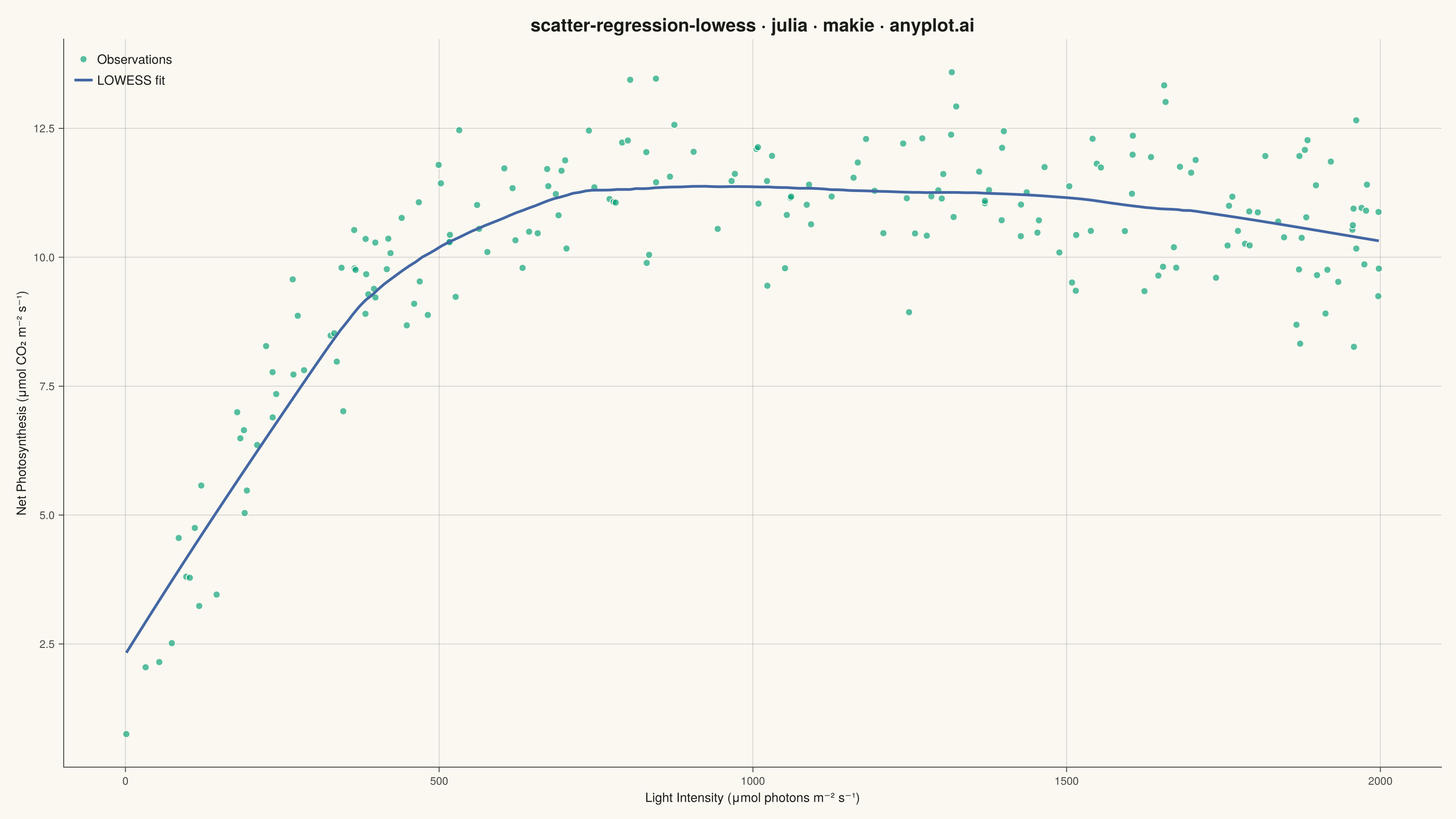
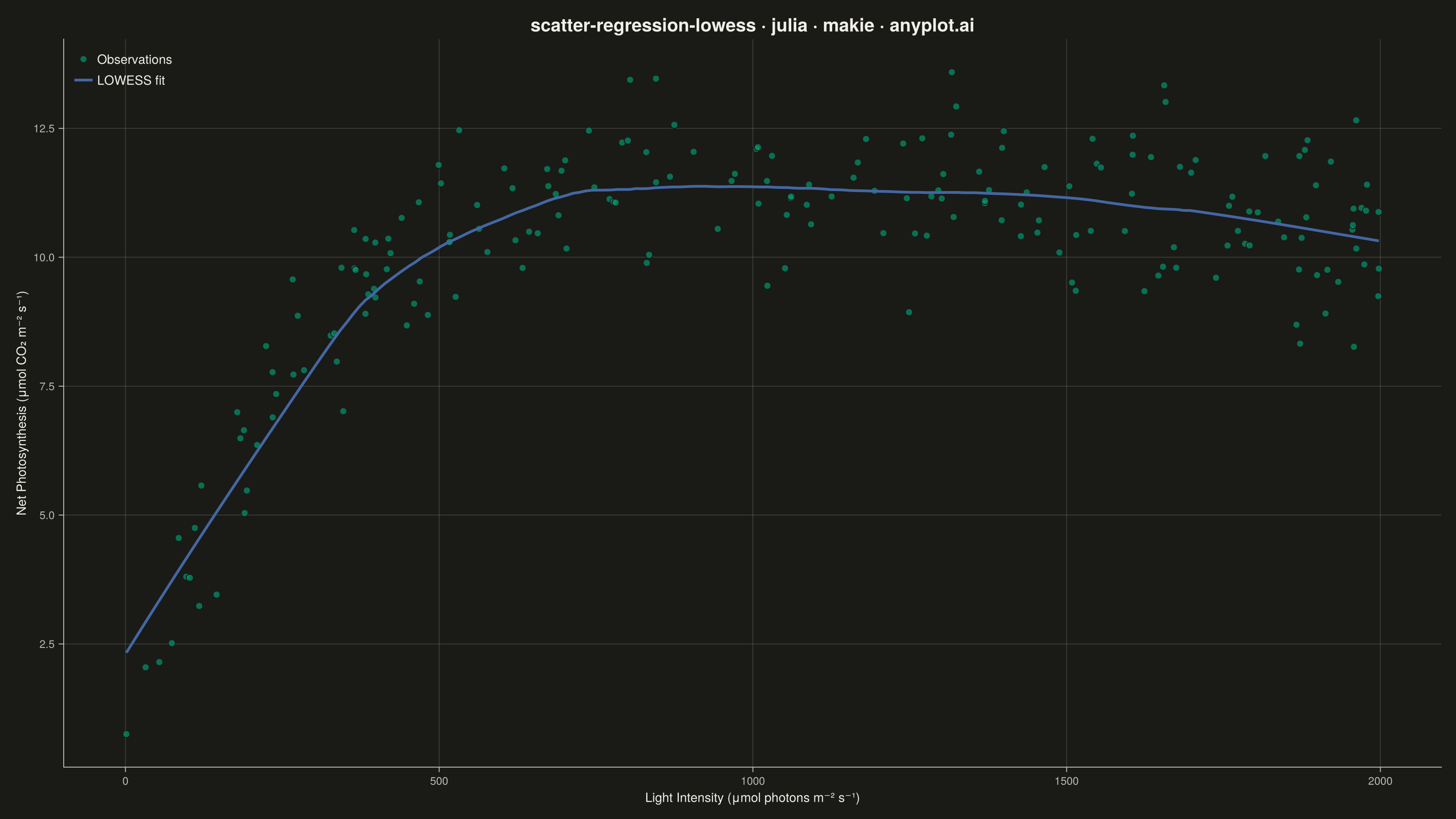
A scatter plot with a LOWESS (Locally Weighted Scatterplot Smoothing) regression curve overlaid. LOWESS is a non-parametric method that fits smooth curves by performing local weighted regressions at each point, adapting to local data patterns without assuming a specific functional form. This makes it ideal for exploring complex relationships where the underlying pattern is unknown or varies across the data range.
# anyplot.ai
# scatter-regression-lowess: Scatter Plot with LOWESS Regression
# Library: makie 0.21.9 | Julia 1.11.9
# Quality: 86/100 | Created: 2026-09-09

using CairoMakie
using Colors
using Random

# --- Theme tokens -------------------------------------------------------------
const THEME       = get(ENV, "ANYPLOT_THEME", "light")
const PAGE_BG     = THEME == "light" ? colorant"#FAF8F1" : colorant"#1A1A17"
const ELEVATED_BG = THEME == "light" ? colorant"#FFFDF6" : colorant"#242420"
const INK         = THEME == "light" ? colorant"#1A1A17" : colorant"#F0EFE8"
const INK_SOFT    = THEME == "light" ? colorant"#4A4A44" : colorant"#B8B7B0"
const BRAND       = colorant"#009E73"  # Imprint palette position 1 — scatter points
const CURVE_COLOR = colorant"#4467A3"  # Imprint palette position 3 — LOWESS fit

# --- Data: light-response curve of net photosynthesis -------------------------
Random.seed!(42)
n = 200
light_intensity = sort(rand(n) .* 2000)  # PAR, μmol photons m⁻² s⁻¹
true_response = 13.5 .* (1 .- exp.(-light_intensity ./ 280)) .- 0.0016 .* light_intensity
net_photosynthesis = true_response .+ randn(n) .* 0.9  # μmol CO2 m⁻² s⁻¹

# --- LOWESS smoothing: local weighted linear regression, tricube weights ------
# A pointwise 95% confidence band is derived from the weighted-regression standard
# error at each evaluation point (weighted residual variance scaled by the local
# effective sample size sw^2 / sum(w^2)).
frac = 0.35
k = ceil(Int, frac * n)
eval_x = collect(range(minimum(light_intensity), maximum(light_intensity); length = 200))
fitted_y = similar(eval_x)
band_lo = similar(eval_x)
band_hi = similar(eval_x)

for (i, x0) in enumerate(eval_x)
    dist = abs.(light_intensity .- x0)
    d_max = sort(dist)[k]
    w = ifelse.(dist .<= d_max, (1 .- clamp.(dist ./ d_max, 0, 1) .^ 3) .^ 3, 0.0)

    sw = sum(w)
    sx = sum(w .* light_intensity)
    sy = sum(w .* net_photosynthesis)
    sxx = sum(w .* light_intensity .^ 2)
    sxy = sum(w .* light_intensity .* net_photosynthesis)

    slope = (sw * sxy - sx * sy) / (sw * sxx - sx^2)
    intercept = (sy - slope * sx) / sw
    fitted_y[i] = intercept + slope * x0

    resid = net_photosynthesis .- (intercept .+ slope .* light_intensity)
    weighted_var = sum(w .* resid .^ 2) / sw
    effective_n = sw^2 / sum(w .^ 2)
    se = sqrt(weighted_var / effective_n)
    band_lo[i] = fitted_y[i] - 1.96 * se
    band_hi[i] = fitted_y[i] + 1.96 * se
end

# --- Plot -----------------------------------------------------------------
fig = Figure(
    resolution      = (1600, 900),
    fontsize        = 14,
    backgroundcolor = PAGE_BG,
)

ax = Axis(
    fig[1, 1];
    title             = "scatter-regression-lowess · julia · makie · anyplot.ai",
    titlesize         = 20,
    titlecolor        = INK,
    xlabel            = "Light Intensity (μmol photons m⁻² s⁻¹)",
    ylabel            = "Net Photosynthesis (μmol CO₂ m⁻² s⁻¹)",
    xlabelsize        = 14,
    ylabelsize        = 14,
    xticklabelsize    = 12,
    yticklabelsize    = 12,
    xlabelcolor       = INK,
    ylabelcolor       = INK,
    xticklabelcolor   = INK_SOFT,
    yticklabelcolor   = INK_SOFT,
    xtickcolor        = INK_SOFT,
    ytickcolor        = INK_SOFT,
    backgroundcolor   = PAGE_BG,
    topspinevisible   = false,
    rightspinevisible = false,
    leftspinecolor    = INK_SOFT,
    bottomspinecolor  = INK_SOFT,
    xgridcolor        = RGBAf(INK.r, INK.g, INK.b, 0.15),
    ygridcolor        = RGBAf(INK.r, INK.g, INK.b, 0.15),
)

band!(ax, eval_x, band_lo, band_hi; color = (CURVE_COLOR, 0.35))
scatter!(
    ax, light_intensity, net_photosynthesis;
    color = (BRAND, 0.55), markersize = 9,
    strokecolor = PAGE_BG, strokewidth = 1,
)
lines!(ax, eval_x, fitted_y; color = CURVE_COLOR, linewidth = 3)

# `band!` has no automatic legend entry in Makie, so the legend is built explicitly
# from proxy elements that mirror the actual plot styling.
legend_elements = [
    MarkerElement(color = (BRAND, 0.55), marker = :circle, markersize = 9, strokecolor = PAGE_BG, strokewidth = 1),
    LineElement(color = CURVE_COLOR, linewidth = 3),
    PolyElement(color = (CURVE_COLOR, 0.35)),
]
legend_labels = ["Observations", "LOWESS fit", "95% CI"]
axislegend(ax, legend_elements, legend_labels; position = :lt, backgroundcolor = ELEVATED_BG, labelcolor = INK, framevisible = false)

# --- Save -------------------------------------------------------------------
save("plot-$(THEME).png", fig; px_per_unit = 2)
Runnable source as JSON, for any HTTP client: https://api.anyplot.ai/specs/scatter-regression-lowess/makie/code. Any spec id and library id listed in llms-full.txt fit the same URL shape; every URL below is complete and callable.
{
  "spec_id": "scatter-regression-lowess",
  "language": "julia",
  "library": "makie",
  "page": "https://anyplot.ai/scatter-regression-lowess/julia/makie",
  "hub": "https://anyplot.ai/scatter-regression-lowess",
  "code_json": "https://api.anyplot.ai/specs/scatter-regression-lowess/makie/code",
  "spec_json": "https://api.anyplot.ai/specs/scatter-regression-lowess",
  "render_light_png": "https://storage.googleapis.com/anyplot-images/plots/scatter-regression-lowess/julia/makie/plot-light.png",
  "render_dark_png": "https://storage.googleapis.com/anyplot-images/plots/scatter-regression-lowess/julia/makie/plot-dark.png",
  "quality_score": 86.0,
  "license": "MIT",
  "guide": "https://anyplot.ai/llms.txt"
}
Part of Scatter Plot with LOWESS Regression on anyplot.ai.