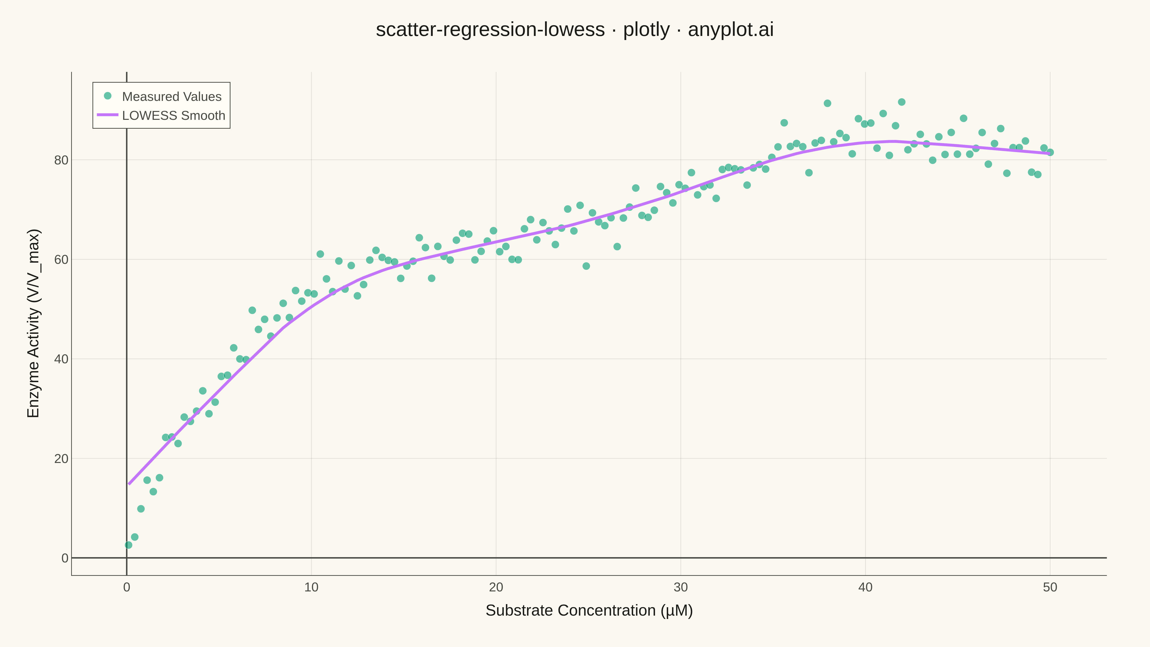
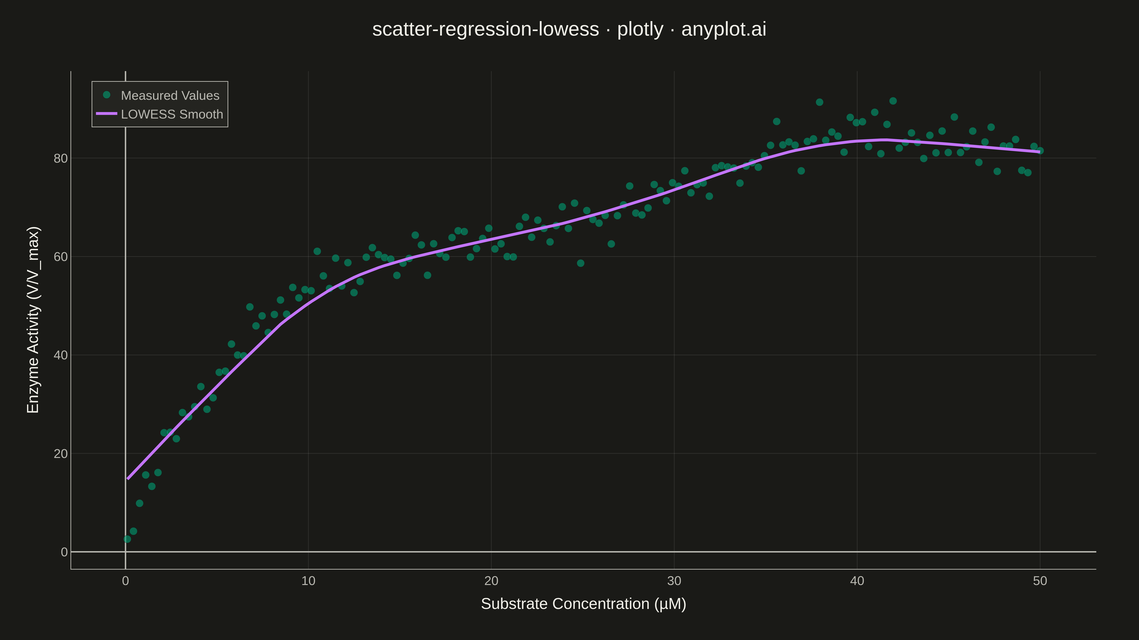
A scatter plot with a LOWESS (Locally Weighted Scatterplot Smoothing) regression curve overlaid. LOWESS is a non-parametric method that fits smooth curves by performing local weighted regressions at each point, adapting to local data patterns without assuming a specific functional form. This makes it ideal for exploring complex relationships where the underlying pattern is unknown or varies across the data range.
""" anyplot.ai
scatter-regression-lowess: Scatter Plot with LOWESS Regression
Library: plotly 6.7.0 | Python 3.13.13
Quality: 84/100 | Updated: 2026-05-14
"""

import os
import numpy as np
import plotly.graph_objects as go
from statsmodels.nonparametric.smoothers_lowess import lowess

# Theme tokens
THEME       = os.getenv("ANYPLOT_THEME", "light")
PAGE_BG     = "#FAF8F1" if THEME == "light" else "#1A1A17"
ELEVATED_BG = "#FFFDF6" if THEME == "light" else "#242420"
INK         = "#1A1A17" if THEME == "light" else "#F0EFE8"
INK_SOFT    = "#4A4A44" if THEME == "light" else "#B8B7B0"
GRID        = "rgba(26,26,23,0.10)" if THEME == "light" else "rgba(240,239,232,0.10)"
BRAND       = "#009E73"  # Okabe-Ito position 1
ACCENT      = "#C475FD"  # Okabe-Ito position 2

# Data - Enzyme kinetics: realistic biological dose-response relationship
# Different structure than seaborn: exponential saturation curve with noise
np.random.seed(42)
n_points = 150
# Substrate concentration (biological domain)
x = np.linspace(0.1, 50, n_points)
# Michaelis-Menten style response: complex saturation with local variations
y = (100 * x) / (10 + x) + np.random.normal(0, 3, n_points) + 5 * np.sin(x / 5)

# Apply LOWESS smoothing using statsmodels
lowess_result = lowess(y, x, frac=0.35, it=3)
x_lowess = lowess_result[:, 0]
y_lowess = lowess_result[:, 1]

# Create figure
fig = go.Figure()

# Add scatter points
fig.add_trace(
    go.Scatter(
        x=x,
        y=y,
        mode="markers",
        name="Measured Values",
        marker=dict(
            size=11,
            color=BRAND,
            opacity=0.6,
            line=dict(color=PAGE_BG, width=0.5),
        ),
    )
)

# Add LOWESS curve
fig.add_trace(
    go.Scatter(
        x=x_lowess,
        y=y_lowess,
        mode="lines",
        name="LOWESS Smooth",
        line=dict(
            color=ACCENT,
            width=4,
        ),
    )
)

# Update layout for large canvas with theme-adaptive styling
fig.update_layout(
    title=dict(
        text="scatter-regression-lowess · plotly · anyplot.ai",
        font=dict(size=28, color=INK),
        x=0.5,
        xanchor="center",
    ),
    xaxis=dict(
        title=dict(text="Substrate Concentration (µM)", font=dict(size=22, color=INK)),
        tickfont=dict(size=18, color=INK_SOFT),
        gridcolor=GRID,
        linecolor=INK_SOFT,
        zerolinecolor=INK_SOFT,
    ),
    yaxis=dict(
        title=dict(text="Enzyme Activity (V/V_max)", font=dict(size=22, color=INK)),
        tickfont=dict(size=18, color=INK_SOFT),
        gridcolor=GRID,
        linecolor=INK_SOFT,
        zerolinecolor=INK_SOFT,
    ),
    paper_bgcolor=PAGE_BG,
    plot_bgcolor=PAGE_BG,
    font=dict(color=INK),
    legend=dict(
        font=dict(size=18, color=INK_SOFT),
        x=0.02,
        y=0.98,
        xanchor="left",
        yanchor="top",
        bgcolor=ELEVATED_BG,
        bordercolor=INK_SOFT,
        borderwidth=1,
    ),
    margin=dict(l=100, r=60, t=100, b=100),
    showlegend=True,
)

# Save as PNG (4800 x 2700 px)
fig.write_image(f"plot-{THEME}.png", width=1600, height=900, scale=3)

# Save as HTML for interactivity
fig.write_html(f"plot-{THEME}.html", include_plotlyjs="cdn")
Runnable source as JSON, for any HTTP client: https://api.anyplot.ai/specs/scatter-regression-lowess/plotly/code. Any spec id and library id listed in llms-full.txt fit the same URL shape; every URL below is complete and callable.
{
  "spec_id": "scatter-regression-lowess",
  "language": "python",
  "library": "plotly",
  "page": "https://anyplot.ai/scatter-regression-lowess/python/plotly",
  "hub": "https://anyplot.ai/scatter-regression-lowess",
  "code_json": "https://api.anyplot.ai/specs/scatter-regression-lowess/plotly/code",
  "spec_json": "https://api.anyplot.ai/specs/scatter-regression-lowess",
  "render_light_png": "https://storage.googleapis.com/anyplot-images/plots/scatter-regression-lowess/python/plotly/plot-light.png",
  "render_dark_png": "https://storage.googleapis.com/anyplot-images/plots/scatter-regression-lowess/python/plotly/plot-dark.png",
  "interactive_light_html": "https://storage.googleapis.com/anyplot-images/plots/scatter-regression-lowess/python/plotly/plot-light.html",
  "interactive_dark_html": "https://storage.googleapis.com/anyplot-images/plots/scatter-regression-lowess/python/plotly/plot-dark.html",
  "quality_score": 84.0,
  "license": "MIT",
  "guide": "https://anyplot.ai/llms.txt"
}
Part of Scatter Plot with LOWESS Regression on anyplot.ai.