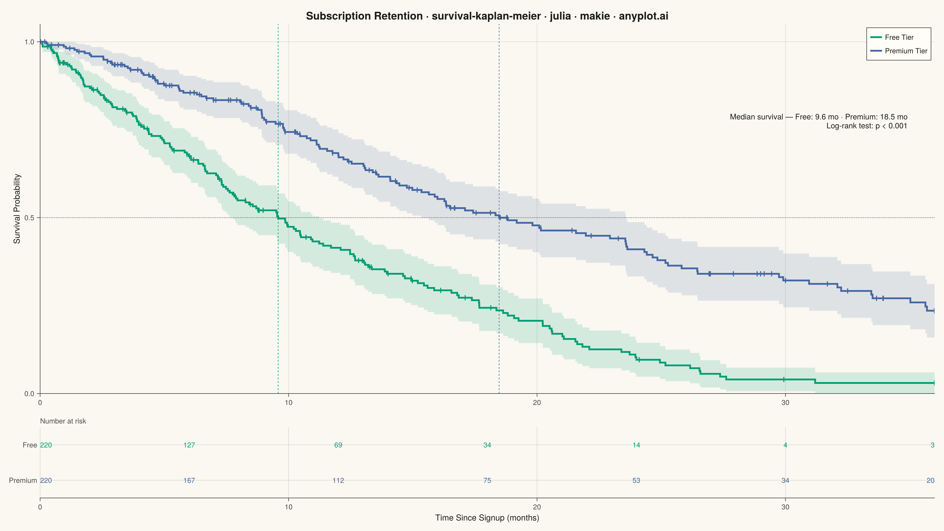
The same plot in 14 other libraries — Python: Altair, Bokeh, lets-plot, Matplotlib, Plotly, plotnine, Pygal, Seaborn; R: ggplot2; JavaScript: Chart.js, D3.js, Apache ECharts, Highcharts, MUI X Charts. Compare all 15 side by side: Kaplan-Meier Survival Plot in Python, R, Julia and JavaScript.
A Kaplan-Meier survival plot visualizes the probability of survival (or event-free time) over a time period using a step function. It is the standard method for estimating survival functions from time-to-event data, handling censored observations where the event has not yet occurred. The plot shows how survival probability decreases over time, with optional confidence intervals and comparison between groups.
# anyplot.ai
# survival-kaplan-meier: Kaplan-Meier Survival Plot
# Library: makie 0.21.9 | Julia 1.11.9
# Quality: 92/100 | Created: 2026-09-09

using CairoMakie
using Colors
using Random

Random.seed!(42)

# Theme tokens
const THEME       = get(ENV, "ANYPLOT_THEME", "light")
const PAGE_BG     = THEME == "light" ? colorant"#FAF8F1" : colorant"#1A1A17"
const ELEVATED_BG = THEME == "light" ? colorant"#FFFDF6" : colorant"#242420"
const INK         = THEME == "light" ? colorant"#1A1A17" : colorant"#F0EFE8"
const INK_SOFT    = THEME == "light" ? colorant"#4A4A44" : colorant"#B8B7B0"

const IMPRINT_PALETTE = [
    colorant"#009E73",
    colorant"#C475FD",
    colorant"#4467A3",
    colorant"#BD8233",
    colorant"#AE3030",
    colorant"#2ABCCD",
    colorant"#954477",
    colorant"#99B314",
]

# Data — subscription retention: Free vs Premium tier time-to-churn (months)
n_free    = 220
n_premium = 220
study_end = 36.0

churn_free     = 14.0 .* (-log.(rand(n_free))) .^ (1 / 1.3)
churn_premium  = 26.0 .* (-log.(rand(n_premium))) .^ (1 / 1.3)
censor_free    = min.(study_end, 40.0 .* (-log.(rand(n_free))))
censor_premium = min.(study_end, 40.0 .* (-log.(rand(n_premium))))

time_free     = min.(churn_free, censor_free)
event_free    = Int.(churn_free .<= censor_free)
time_premium  = min.(churn_premium, censor_premium)
event_premium = Int.(churn_premium .<= censor_premium)

# Kaplan-Meier estimator with Greenwood's formula for the standard error
function kaplan_meier(time, event)
    event_times = sort(unique(time[event .== 1]))
    survival = Float64[]
    stderr   = Float64[]

    s = 1.0
    greenwood_sum = 0.0
    for et in event_times
        n_risk = count(>=(et), time)
        d      = count(==(et), time[event .== 1])
        s *= (1 - d / n_risk)
        push!(survival, s)
        if n_risk > d
            greenwood_sum += d / (n_risk * (n_risk - d))
        end
        push!(stderr, s * sqrt(greenwood_sum))
    end

    censor_times = time[event .== 0]
    return event_times, survival, stderr, censor_times
end

# Step-function coordinates for the curve and its 95% confidence band
function km_step(event_times, survival, stderr, t_start, t_end)
    xs, ys, lo, hi = Float64[t_start], Float64[1.0], Float64[1.0], Float64[1.0]
    for i in eachindex(event_times)
        push!(xs, event_times[i]); push!(ys, ys[end]); push!(lo, lo[end]); push!(hi, hi[end])
        push!(xs, event_times[i]); push!(ys, survival[i])
        push!(lo, clamp(survival[i] - 1.96 * stderr[i], 0.0, 1.0))
        push!(hi, clamp(survival[i] + 1.96 * stderr[i], 0.0, 1.0))
    end
    push!(xs, t_end); push!(ys, ys[end]); push!(lo, lo[end]); push!(hi, hi[end])
    return xs, ys, lo, hi
end

survival_at(event_times, survival, t) = isempty(event_times) || t < event_times[1] ? 1.0 :
    survival[findlast(<=(t), event_times)]

et_free, surv_free, se_free, cens_free = kaplan_meier(time_free, event_free)
et_prem, surv_prem, se_prem, cens_prem = kaplan_meier(time_premium, event_premium)

xs_free, ys_free, lo_free, hi_free = km_step(et_free, surv_free, se_free, 0.0, study_end)
xs_prem, ys_prem, lo_prem, hi_prem = km_step(et_prem, surv_prem, se_prem, 0.0, study_end)

cens_y_free = [survival_at(et_free, surv_free, t) for t in cens_free]
cens_y_prem = [survival_at(et_prem, surv_prem, t) for t in cens_prem]

median_idx_free = findfirst(<=(0.5), surv_free)
median_idx_prem = findfirst(<=(0.5), surv_prem)
median_free = median_idx_free === nothing ? nothing : et_free[median_idx_free]
median_prem = median_idx_prem === nothing ? nothing : et_prem[median_idx_prem]

# Log-rank test (Mantel-Haenszel chi-square, 1 df) comparing the two groups
combined_event_times = sort(unique(vcat(et_free, et_prem)))
observed_free, expected_free, variance_sum = 0.0, 0.0, 0.0
for t in combined_event_times
    n1 = count(>=(t), time_free)
    n2 = count(>=(t), time_premium)
    d1 = count(==(t), time_free[event_free .== 1])
    d2 = count(==(t), time_premium[event_premium .== 1])
    n, d = n1 + n2, d1 + d2
    if n > 1 && d > 0
        global observed_free += d1
        global expected_free += d * n1 / n
        global variance_sum += d * (n1 / n) * (n2 / n) * ((n - d) / (n - 1))
    end
end
logrank_chi2 = (observed_free - expected_free)^2 / variance_sum

# Standard normal CDF (Abramowitz & Stegun 26.2.17) — avoids a SpecialFunctions dependency
function normal_cdf(x)
    z = abs(x)
    t = 1 / (1 + 0.2316419 * z)
    poly = t * (0.319381530 + t * (-0.356563782 + t * (1.781477937 +
           t * (-1.821255978 + t * 1.330274429))))
    phi = 1 - poly * exp(-z^2 / 2) / sqrt(2π)
    return x >= 0 ? phi : 1 - phi
end
logrank_p = 2 * (1 - normal_cdf(sqrt(logrank_chi2)))

# Number-at-risk table gridpoints
risk_times = collect(0.0:6.0:study_end)
risk_free  = [count(>=(t), time_free) for t in risk_times]
risk_prem  = [count(>=(t), time_premium) for t in risk_times]

# Title (scaled fontsize — descriptive prefix pushes past the 67-char baseline)
title_str  = "Subscription Retention · survival-kaplan-meier · julia · makie · anyplot.ai"
title_size = max(14, round(Int, 20 * min(1.0, 67.0 / length(title_str))))

# Plot
fig = Figure(
    size            = (1600, 900),
    fontsize        = 14,
    backgroundcolor = PAGE_BG,
)

ax = Axis(
    fig[1, 1];
    title             = title_str,
    titlesize         = title_size,
    titlecolor        = INK,
    ylabel            = "Survival Probability",
    xlabelsize        = 14,
    ylabelsize        = 14,
    xticklabelsize    = 12,
    yticklabelsize    = 12,
    xlabelcolor       = INK,
    ylabelcolor       = INK,
    xticklabelcolor   = INK_SOFT,
    yticklabelcolor   = INK_SOFT,
    xtickcolor        = INK_SOFT,
    ytickcolor        = INK_SOFT,
    backgroundcolor   = PAGE_BG,
    topspinevisible   = false,
    rightspinevisible = false,
    leftspinecolor    = INK_SOFT,
    bottomspinecolor  = INK_SOFT,
    xgridcolor        = RGBAf(INK.r, INK.g, INK.b, 0.12),
    ygridcolor        = RGBAf(INK.r, INK.g, INK.b, 0.12),
    xminorgridvisible = false,
    yminorgridvisible = false,
    limits            = (0.0, study_end, 0.0, 1.05),
)

# 95% confidence bands (Greenwood's formula) — drawn first, behind the curves
band!(ax, xs_free, lo_free, hi_free;
    color = RGBAf(IMPRINT_PALETTE[1].r, IMPRINT_PALETTE[1].g, IMPRINT_PALETTE[1].b, 0.15))
band!(ax, xs_prem, lo_prem, hi_prem;
    color = RGBAf(IMPRINT_PALETTE[2].r, IMPRINT_PALETTE[2].g, IMPRINT_PALETTE[2].b, 0.15))

# Kaplan-Meier step curves
lines!(ax, xs_free, ys_free; color = IMPRINT_PALETTE[1], linewidth = 3.0, label = "Free Tier")
lines!(ax, xs_prem, ys_prem; color = IMPRINT_PALETTE[2], linewidth = 3.0, label = "Premium Tier")

# Censoring marks
scatter!(ax, cens_free, cens_y_free;
    marker = :vline, markersize = 14, color = IMPRINT_PALETTE[1], strokewidth = 0)
scatter!(ax, cens_prem, cens_y_prem;
    marker = :vline, markersize = 14, color = IMPRINT_PALETTE[2], strokewidth = 0)

# Median survival reference lines
hlines!(ax, [0.5]; color = INK_SOFT, linewidth = 1.0, linestyle = :dot)
median_free !== nothing && vlines!(ax, [median_free]; color = IMPRINT_PALETTE[1], linewidth = 1.0, linestyle = :dash)
median_prem !== nothing && vlines!(ax, [median_prem]; color = IMPRINT_PALETTE[2], linewidth = 1.0, linestyle = :dash)

median_free_str = median_free === nothing ? "not reached" : "$(round(median_free; digits = 1)) mo"
median_prem_str = median_prem === nothing ? "not reached" : "$(round(median_prem; digits = 1)) mo"
p_str = logrank_p < 0.001 ? "p < 0.001" : "p = $(round(logrank_p; digits = 3))"

text!(ax,
    "Median survival — Free: $(median_free_str) · Premium: $(median_prem_str)\nLog-rank test: $(p_str)";
    position = Point2f(study_end * 0.97, 0.8),
    align    = (:right, :top),
    color    = INK,
    fontsize = 13,
)

axislegend(ax;
    position        = :rt,
    labelsize       = 12,
    framevisible    = true,
    framecolor      = INK_SOFT,
    backgroundcolor = ELEVATED_BG,
    labelcolor      = INK,
)

# Number-at-risk table
ax_risk = Axis(
    fig[2, 1];
    backgroundcolor     = PAGE_BG,
    limits              = (0.0, study_end, 0.0, 2.0),
    xlabel              = "Time Since Signup (months)",
    xlabelsize          = 14,
    xlabelcolor         = INK,
    xticklabelsize      = 12,
    xticklabelcolor     = INK_SOFT,
    xtickcolor          = INK_SOFT,
    yticks              = ([0.5, 1.5], ["Premium", "Free"]),
    yticklabelsize      = 12,
    yticklabelcolor     = INK_SOFT,
    yticksvisible       = false,
    topspinevisible     = false,
    rightspinevisible   = false,
    leftspinevisible    = false,
    bottomspinecolor    = INK_SOFT,
)
Label(fig[2, 1, Top()], "Number at risk";
    fontsize = 12, color = INK_SOFT, halign = :left, padding = (0, 0, 4, 0))

for (i, t) in enumerate(risk_times)
    halign = i == 1 ? :left : i == length(risk_times) ? :right : :center
    text!(ax_risk, string(risk_free[i]);
        position = Point2f(t, 1.5), align = (halign, :center), color = IMPRINT_PALETTE[1], fontsize = 12)
    text!(ax_risk, string(risk_prem[i]);
        position = Point2f(t, 0.5), align = (halign, :center), color = IMPRINT_PALETTE[2], fontsize = 12)
end

rowsize!(fig.layout, 2, Relative(0.16))

# Save
save("plot-$(THEME).png", fig; px_per_unit = 2)
Runnable source as JSON, for any HTTP client: https://api.anyplot.ai/specs/survival-kaplan-meier/makie/code. Any spec id and library id listed in llms-full.txt fit the same URL shape; every URL below is complete and callable.
{
  "spec_id": "survival-kaplan-meier",
  "language": "julia",
  "library": "makie",
  "page": "https://anyplot.ai/survival-kaplan-meier/julia/makie",
  "hub": "https://anyplot.ai/survival-kaplan-meier",
  "code_json": "https://api.anyplot.ai/specs/survival-kaplan-meier/makie/code",
  "spec_json": "https://api.anyplot.ai/specs/survival-kaplan-meier",
  "render_light_png": "https://storage.googleapis.com/anyplot-images/plots/survival-kaplan-meier/julia/makie/plot-light.png",
  "render_dark_png": "https://storage.googleapis.com/anyplot-images/plots/survival-kaplan-meier/julia/makie/plot-dark.png",
  "quality_score": 92.0,
  "license": "MIT",
  "guide": "https://anyplot.ai/llms.txt"
}
Part of Kaplan-Meier Survival Plot on anyplot.ai.