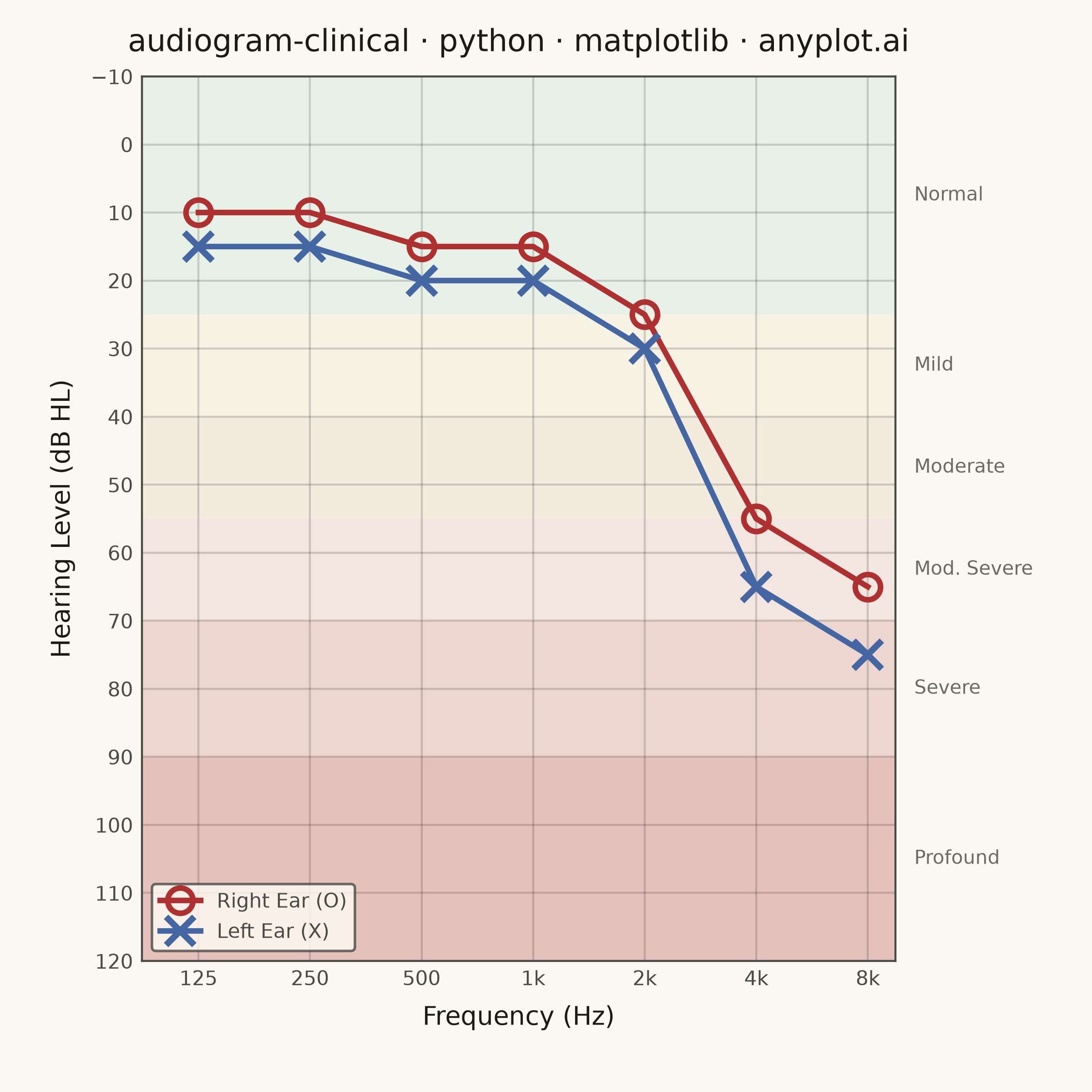
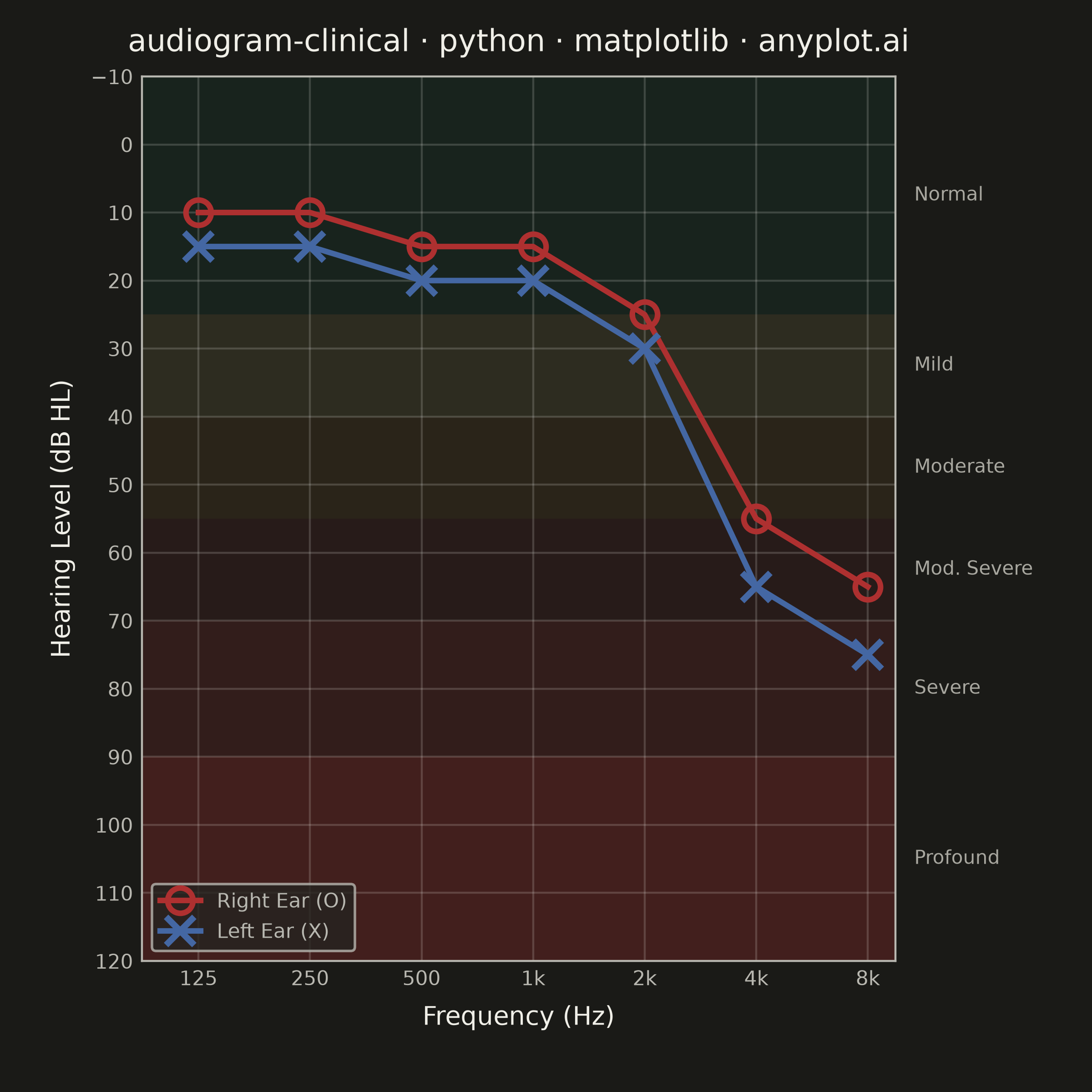
A standardized clinical audiogram that displays hearing test results, plotting hearing threshold (dB HL) against test frequency for each ear. The y-axis is inverted so that 0 dB HL (best hearing) sits at the top and increasing hearing loss extends downward, while the x-axis is logarithmic spanning the standard audiometric frequencies (125 Hz to 8 kHz). Thresholds are marked with the conventional symbols — a circle (O) for the right ear in red and a cross (X) for the left ear in blue — and connected per ear, with shaded horizontal bands indicating severity of hearing loss (normal, mild, moderate, severe, profound).
""" anyplot.ai
audiogram-clinical: Clinical Audiogram
Library: matplotlib 3.11.0 | Python 3.13.13
Quality: 91/100 | Created: 2026-06-14
"""

import sys


# Prevent this file from shadowing the installed matplotlib package when run
# from its own directory (sys.path[0] would otherwise resolve to this file).
sys.path.pop(0)

import os

import matplotlib.pyplot as plt
import matplotlib.ticker as ticker
from matplotlib.transforms import blended_transform_factory


# Theme tokens (see prompts/default-style-guide.md "Theme-adaptive Chrome")
THEME = os.getenv("ANYPLOT_THEME", "light")
PAGE_BG = "#FAF8F1" if THEME == "light" else "#1A1A17"
ELEVATED_BG = "#FFFDF6" if THEME == "light" else "#242420"
INK = "#1A1A17" if THEME == "light" else "#F0EFE8"
INK_SOFT = "#4A4A44" if THEME == "light" else "#B8B7B0"
INK_MUTED = "#6B6A63" if THEME == "light" else "#A8A79F"

# Ear colors — semantic exception from Imprint palette (red=right, blue=left per audiological convention)
RIGHT_EAR = "#AE3030"  # Imprint matte red — right-ear convention
LEFT_EAR = "#4467A3"  # Imprint blue — left-ear convention

# Data — noise-induced high-frequency sensorineural hearing loss (occupational pattern)
frequencies = [125, 250, 500, 1000, 2000, 4000, 8000]
threshold_right = [10, 10, 15, 15, 25, 55, 65]  # right ear (dB HL)
threshold_left = [15, 15, 20, 20, 30, 65, 75]  # left ear (dB HL)

# Severity bands: (y_start, y_end, fill_color, alpha, label)
severity_bands = [
    (-10, 25, "#009E73", 0.07, "Normal"),
    (25, 40, "#DDCC77", 0.10, "Mild"),
    (40, 55, "#BD8233", 0.10, "Moderate"),
    (55, 70, "#AE3030", 0.09, "Mod. Severe"),
    (70, 90, "#AE3030", 0.17, "Severe"),
    (90, 120, "#AE3030", 0.27, "Profound"),
]

# Plot — square canvas for standardized audiogram layout
fig, ax = plt.subplots(figsize=(6, 6), dpi=400, facecolor=PAGE_BG)
ax.set_facecolor(PAGE_BG)

# Severity band shading
for y_start, y_end, color, alpha, _ in severity_bands:
    ax.axhspan(y_start, y_end, alpha=alpha, color=color, zorder=0, lw=0)

# Band labels on right margin outside axes
band_trans = blended_transform_factory(ax.transAxes, ax.transData)
for y_start, y_end, _, _, label in severity_bands:
    mid = (y_start + y_end) / 2
    ax.text(
        1.025, mid, label, transform=band_trans, fontsize=7.5, color=INK_MUTED, va="center", ha="left", clip_on=False
    )

# Right ear — open circle (O) markers with solid connecting line
ax.plot(
    frequencies,
    threshold_right,
    marker="o",
    linestyle="-",
    color=RIGHT_EAR,
    linewidth=2.2,
    markersize=10,
    markerfacecolor="none",
    markeredgewidth=2.2,
    markeredgecolor=RIGHT_EAR,
    label="Right Ear (O)",
    zorder=3,
)

# Left ear — cross (X) markers with solid connecting line
ax.plot(
    frequencies,
    threshold_left,
    marker="x",
    linestyle="-",
    color=LEFT_EAR,
    linewidth=2.2,
    markersize=11,
    markeredgewidth=2.5,
    label="Left Ear (X)",
    zorder=3,
)

# X-axis — logarithmic, standard audiometric frequencies
ax.set_xscale("log")
ax.set_xlim(88, 9500)
ax.set_xticks(frequencies)
ax.set_xticklabels(["125", "250", "500", "1k", "2k", "4k", "8k"])
ax.xaxis.set_minor_locator(ticker.NullLocator())

# Y-axis — inverted (0 dB HL at top), range -10 to 120, gridlines every 10 dB
ax.set_ylim(120, -10)
ax.set_yticks(range(-10, 130, 10))

# Grid — every 10 dB and at each standard frequency
ax.grid(True, which="major", alpha=0.18, linewidth=0.8, color=INK, zorder=1)

# Title with scaled fontsize
title = "audiogram-clinical · python · matplotlib · anyplot.ai"
n = len(title)
title_fs = max(8, round(12 * 67 / n)) if n > 67 else 12

# Chrome styling
ax.set_title(title, fontsize=title_fs, fontweight="medium", color=INK, pad=10)
ax.set_xlabel("Frequency (Hz)", fontsize=10, color=INK, labelpad=6)
ax.set_ylabel("Hearing Level (dB HL)", fontsize=10, color=INK, labelpad=6)
ax.tick_params(axis="both", labelsize=8, colors=INK_SOFT, length=0)

for spine in ax.spines.values():
    spine.set_color(INK_SOFT)
    spine.set_linewidth(0.8)

# Legend — placed in lower-left (high dB HL region, no data)
leg = ax.legend(fontsize=8, loc="lower left")
leg.get_frame().set_facecolor(ELEVATED_BG)
leg.get_frame().set_edgecolor(INK_SOFT)
plt.setp(leg.get_texts(), color=INK_SOFT)

# Layout — explicit margins so severity labels on the right are not clipped
fig.subplots_adjust(left=0.13, right=0.82, top=0.93, bottom=0.12)

# Save
plt.savefig(f"plot-{THEME}.png", dpi=400, facecolor=PAGE_BG)
plt.close()
Runnable source as JSON, for any HTTP client: https://api.anyplot.ai/specs/audiogram-clinical/matplotlib/code. Any spec id and library id listed in llms-full.txt fit the same URL shape; every URL below is complete and callable.
{
  "spec_id": "audiogram-clinical",
  "language": "python",
  "library": "matplotlib",
  "page": "https://anyplot.ai/audiogram-clinical/python/matplotlib",
  "hub": "https://anyplot.ai/audiogram-clinical",
  "code_json": "https://api.anyplot.ai/specs/audiogram-clinical/matplotlib/code",
  "spec_json": "https://api.anyplot.ai/specs/audiogram-clinical",
  "render_light_png": "https://storage.googleapis.com/anyplot-images/plots/audiogram-clinical/python/matplotlib/plot-light.png",
  "render_dark_png": "https://storage.googleapis.com/anyplot-images/plots/audiogram-clinical/python/matplotlib/plot-dark.png",
  "quality_score": 91.0,
  "license": "MIT",
  "guide": "https://anyplot.ai/llms.txt"
}
Part of Clinical Audiogram on anyplot.ai.