The same plot in 14 other libraries — Python: Bokeh, lets-plot, Matplotlib, Plotly, plotnine, Pygal, Seaborn; R: ggplot2; Julia: Makie.jl; JavaScript: Chart.js, D3.js, Apache ECharts, Highcharts, MUI X Charts. Compare all 15 side by side: Bias-Variance Tradeoff Curve in Python, R, Julia and JavaScript.
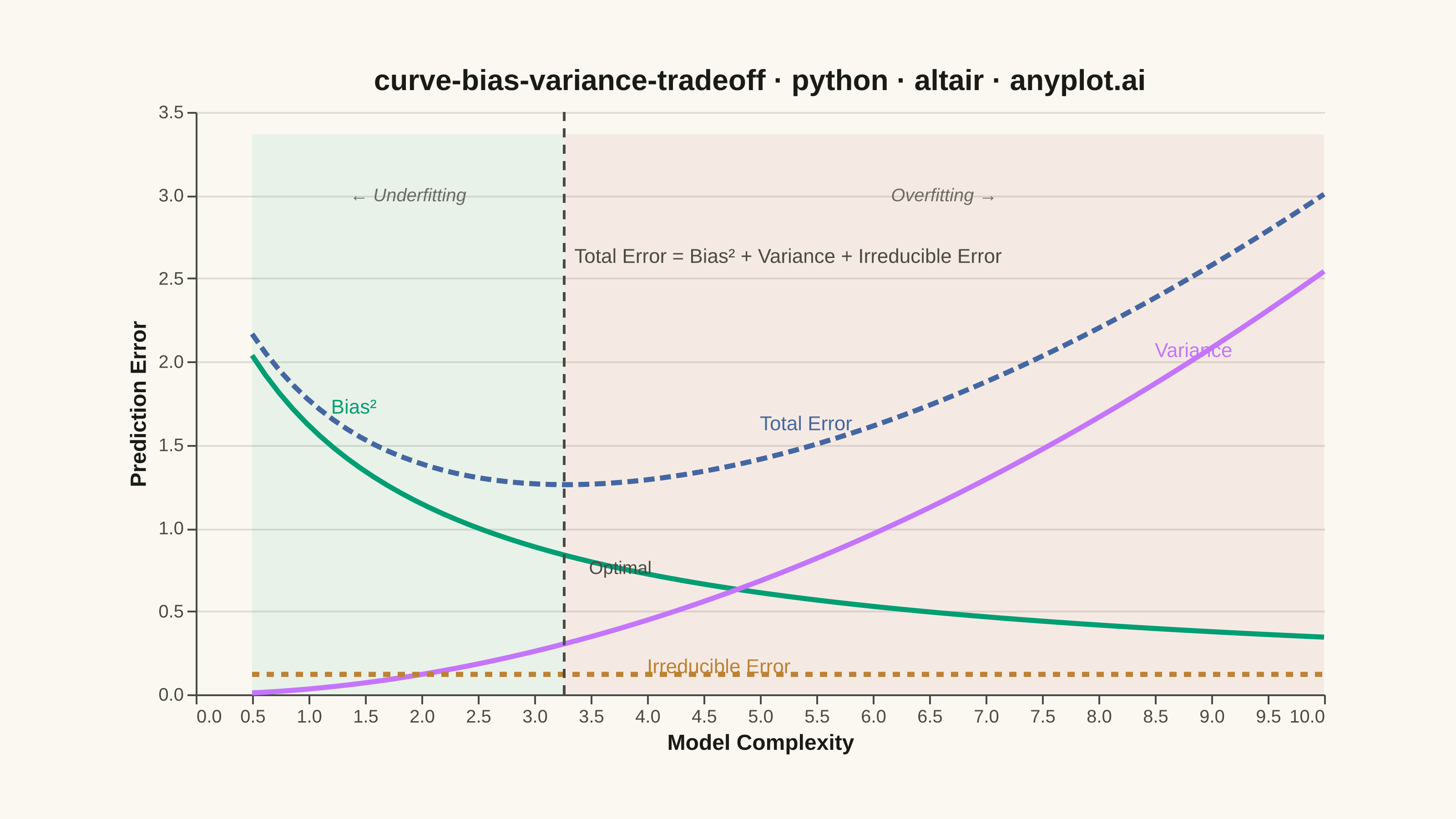
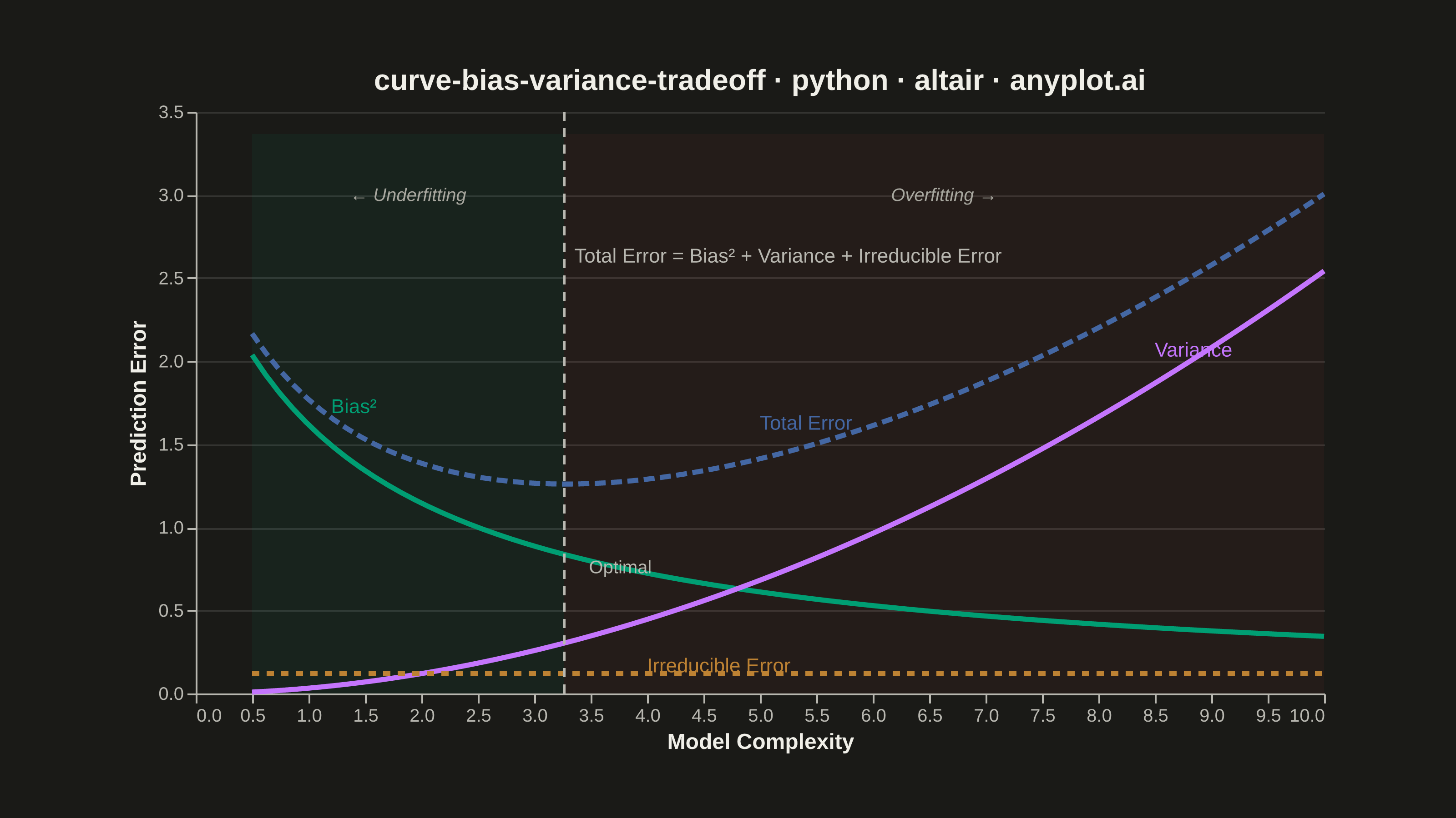
A theoretical visualization of the bias-variance tradeoff showing how total prediction error decomposes into bias squared, variance, and irreducible noise as a function of model complexity. The plot displays multiple curves: bias squared (decreasing with complexity), variance (increasing with complexity), irreducible error (constant), and total error (U-shaped). This is one of the most fundamental conceptual plots in machine learning for understanding model selection, overfitting, and underfitting.
""" anyplot.ai
curve-bias-variance-tradeoff: Bias-Variance Tradeoff Curve
Library: altair 6.1.0 | Python 3.13.13
Quality: 90/100 | Created: 2026-05-28
"""

import os
import sys


# Prevent self-import: this file is named altair.py, so remove its directory
# from sys.path before importing the altair package.
_this_dir = os.path.dirname(os.path.abspath(__file__))
sys.path = [p for p in sys.path if p and os.path.abspath(p) != _this_dir]

import altair as alt
import numpy as np
import pandas as pd
from PIL import Image


# Theme tokens
THEME = os.getenv("ANYPLOT_THEME", "light")
PAGE_BG = "#FAF8F1" if THEME == "light" else "#1A1A17"
ELEVATED_BG = "#FFFDF6" if THEME == "light" else "#242420"
INK = "#1A1A17" if THEME == "light" else "#F0EFE8"
INK_SOFT = "#4A4A44" if THEME == "light" else "#B8B7B0"
INK_MUTED = "#6B6A63" if THEME == "light" else "#A8A79F"

IMPRINT_PALETTE = ["#009E73", "#C475FD", "#4467A3", "#BD8233", "#AE3030", "#2ABCCD", "#954477", "#99B314"]

# Data — theoretical bias-variance tradeoff curves
np.random.seed(42)
n = 80
complexity = np.linspace(0.5, 10.0, n)

bias_sq = 1.1 / (0.4 + complexity * 0.28)
variance = 0.032 * complexity**1.9
irr_error = np.full(n, 0.12)
total_error = bias_sq + variance + irr_error

opt_idx = int(np.argmin(total_error))
opt_complexity = float(complexity[opt_idx])
y_max = float(total_error.max()) * 1.12

# Long-form data for lines
curve_names = ["Bias²", "Variance", "Total Error", "Irreducible Error"]
curve_vals = [bias_sq, variance, total_error, irr_error]
rows = []
for name, vals in zip(curve_names, curve_vals, strict=True):
    for c, v in zip(complexity, vals, strict=True):
        rows.append({"complexity": float(c), "error": float(v), "curve": name})
df = pd.DataFrame(rows)

color_domain = curve_names
color_range = IMPRINT_PALETTE[:4]
dash_domain = curve_names
dash_range = [[1, 0], [1, 0], [6, 3], [4, 4]]

# Shaded regions — two separate dataframes, each with a fixed color, to avoid
# merging their color channel with the lines layer's color encoding.
shade_under_df = pd.DataFrame([{"complexity": 0.5, "complexity_end": opt_complexity, "error": 0.0, "error_end": y_max}])
shade_over_df = pd.DataFrame([{"complexity": opt_complexity, "complexity_end": 10.0, "error": 0.0, "error_end": y_max}])

# Direct curve labels
label_df = pd.DataFrame(
    [
        {"complexity": 1.2, "error": 1.72, "label": "Bias²", "curve": "Bias²"},
        {"complexity": 8.5, "error": 2.06, "label": "Variance", "curve": "Variance"},
        {"complexity": 5.0, "error": 1.62, "label": "Total Error", "curve": "Total Error"},
        {"complexity": 4.0, "error": 0.16, "label": "Irreducible Error", "curve": "Irreducible Error"},
    ]
)

# Optimal complexity rule
opt_df = pd.DataFrame({"complexity": [opt_complexity]})

# Optimal label
opt_label_df = pd.DataFrame(
    [{"complexity": opt_complexity + 0.22, "error": float(total_error[opt_idx]) * 0.60, "text": "Optimal"}]
)

# Zone labels
zone_df = pd.DataFrame(
    [
        {"complexity": (0.5 + opt_complexity) / 2, "error": y_max * 0.89, "text": "← Underfitting"},
        {"complexity": (opt_complexity + 10.0) / 2, "error": y_max * 0.89, "text": "Overfitting →"},
    ]
)

# Formula annotation
formula_df = pd.DataFrame(
    [{"complexity": 5.25, "error": y_max * 0.78, "text": "Total Error = Bias² + Variance + Irreducible Error"}]
)

title = "curve-bias-variance-tradeoff · python · altair · anyplot.ai"
x_scale = alt.Scale(domain=[0.5, 10.0])
y_scale = alt.Scale(domain=[0.0, y_max])

# Layer 1: Shaded zones — fixed fill colors to avoid merging with lines scale
shade_under_layer = (
    alt.Chart(shade_under_df)
    .mark_rect(fill=IMPRINT_PALETTE[0], opacity=0.07, stroke=None)
    .encode(
        x=alt.X("complexity:Q", scale=x_scale),
        x2="complexity_end:Q",
        y=alt.Y("error:Q", scale=y_scale),
        y2="error_end:Q",
    )
)
shade_over_layer = (
    alt.Chart(shade_over_df)
    .mark_rect(fill=IMPRINT_PALETTE[4], opacity=0.07, stroke=None)
    .encode(
        x=alt.X("complexity:Q", scale=x_scale),
        x2="complexity_end:Q",
        y=alt.Y("error:Q", scale=y_scale),
        y2="error_end:Q",
    )
)

# Layer 2: Curves
lines_layer = (
    alt.Chart(df)
    .mark_line(strokeWidth=2.8)
    .encode(
        x=alt.X("complexity:Q", title="Model Complexity", scale=x_scale),
        y=alt.Y("error:Q", title="Prediction Error", scale=y_scale),
        color=alt.Color("curve:N", scale=alt.Scale(domain=color_domain, range=color_range), legend=None),
        strokeDash=alt.StrokeDash("curve:N", scale=alt.Scale(domain=dash_domain, range=dash_range), legend=None),
    )
)

# Layer 3: Optimal complexity vertical rule
opt_rule_layer = (
    alt.Chart(opt_df).mark_rule(strokeDash=[5, 4], strokeWidth=1.5, color=INK_SOFT).encode(x="complexity:Q")
)

# Layer 4: Curve labels
label_layer = (
    alt.Chart(label_df)
    .mark_text(fontSize=11, align="left", fontWeight="normal")
    .encode(
        x="complexity:Q",
        y="error:Q",
        text="label:N",
        color=alt.Color("curve:N", scale=alt.Scale(domain=color_domain, range=color_range), legend=None),
    )
)

# Layer 5: Zone labels
zone_layer = (
    alt.Chart(zone_df)
    .mark_text(fontSize=10, color=INK_MUTED, fontStyle="italic")
    .encode(x="complexity:Q", y="error:Q", text="text:N")
)

# Layer 6: Optimal label
opt_label_layer = (
    alt.Chart(opt_label_df)
    .mark_text(fontSize=10, align="left", color=INK_SOFT)
    .encode(x="complexity:Q", y="error:Q", text="text:N")
)

# Layer 7: Formula
formula_layer = (
    alt.Chart(formula_df).mark_text(fontSize=11, color=INK_SOFT).encode(x="complexity:Q", y="error:Q", text="text:N")
)

chart = (
    alt.layer(
        shade_under_layer,
        shade_over_layer,
        lines_layer,
        opt_rule_layer,
        label_layer,
        zone_layer,
        opt_label_layer,
        formula_layer,
    )
    .properties(width=620, height=320, background=PAGE_BG, title=alt.TitleParams(text=title, fontSize=16, color=INK))
    .configure_view(fill=PAGE_BG, stroke=None)
    .configure_axis(
        domainColor=INK_SOFT,
        tickColor=INK_SOFT,
        gridColor=INK,
        gridOpacity=0.12,
        labelColor=INK_SOFT,
        labelFontSize=10,
        titleColor=INK,
        titleFontSize=12,
    )
    .configure_axisX(grid=False)
    .configure_legend(
        fillColor=ELEVATED_BG,
        strokeColor=INK_SOFT,
        labelColor=INK_SOFT,
        titleColor=INK,
        labelFontSize=10,
        titleFontSize=10,
    )
)

# Save PNG
chart.save(f"plot-{THEME}.png", scale_factor=4.0)

# Pad to exact target dimensions (3200 × 1800)
TW, TH = 3200, 1800
_img = Image.open(f"plot-{THEME}.png").convert("RGB")
_w, _h = _img.size
if _w > TW or _h > TH:
    raise SystemExit(
        f"altair vl-convert produced {_w}×{_h}, exceeds target {TW}×{TH}. "
        "Shrink chart .properties(width=, height=) values and re-render."
    )
if _w < TW or _h < TH:
    _canvas = Image.new("RGB", (TW, TH), PAGE_BG)
    _canvas.paste(_img, ((TW - _w) // 2, (TH - _h) // 2))
    _canvas.save(f"plot-{THEME}.png")

# Save HTML
chart.save(f"plot-{THEME}.html")
Runnable source as JSON, for any HTTP client: https://api.anyplot.ai/specs/curve-bias-variance-tradeoff/altair/code. Any spec id and library id listed in llms-full.txt fit the same URL shape; every URL below is complete and callable.
{
  "spec_id": "curve-bias-variance-tradeoff",
  "language": "python",
  "library": "altair",
  "page": "https://anyplot.ai/curve-bias-variance-tradeoff/python/altair",
  "hub": "https://anyplot.ai/curve-bias-variance-tradeoff",
  "code_json": "https://api.anyplot.ai/specs/curve-bias-variance-tradeoff/altair/code",
  "spec_json": "https://api.anyplot.ai/specs/curve-bias-variance-tradeoff",
  "render_light_png": "https://storage.googleapis.com/anyplot-images/plots/curve-bias-variance-tradeoff/python/altair/plot-light.png",
  "render_dark_png": "https://storage.googleapis.com/anyplot-images/plots/curve-bias-variance-tradeoff/python/altair/plot-dark.png",
  "interactive_light_html": "https://storage.googleapis.com/anyplot-images/plots/curve-bias-variance-tradeoff/python/altair/plot-light.html",
  "interactive_dark_html": "https://storage.googleapis.com/anyplot-images/plots/curve-bias-variance-tradeoff/python/altair/plot-dark.html",
  "quality_score": 90.0,
  "license": "MIT",
  "guide": "https://anyplot.ai/llms.txt"
}
Part of Bias-Variance Tradeoff Curve on anyplot.ai.